What are Correlation Coefficients?
Correlation coefficients measure the strength of the relationship between two variables. A correlation between variables indicates that as one variable changes in value, the other variable tends to change in a specific direction. Understanding that relationship is useful because we can use the value of one variable to predict the value of the other variable. For example, height and weight are correlated—as height increases, weight also tends to increase. Consequently, if we observe an individual who is unusually tall, we can predict that his weight is also above the average.
In statistical analysis, correlation coefficients are a quantitative assessment that measures both the direction and the strength of this tendency to vary together. There are different types of correlation coefficients that you can use for different kinds of data. In this post, I cover the most common type of correlation—Pearson’s correlation coefficient.
Before we get into the numbers, let’s graph some data first so we can understand the concept behind what we are measuring.
Graph Your Data to Find Correlations
Scatterplots are a great way to check quickly for correlation between pairs of continuous data. The scatterplot below displays the height and weight of pre-teenage girls. Each dot on the graph represents an individual girl and her combination of height and weight. These data are actual data that I collected during an experiment.

At a glance, you can see that there is a correlation between height and weight. As height increases, weight also tends to increase. However, it’s not a perfect relationship. If you look at a specific height, say 1.5 meters, you can see that there is a range of weights associated with it. You can also find short people who weigh more than taller people. However, the general tendency that height and weight increase together is unquestionably present—a correlation exists.
Pearson’s correlation coefficient takes all of the data points on this graph and represents them as a single number. In this case, the statistical output below indicates that the Pearson’s correlation coefficient is 0.694.

What do the Pearson correlation coefficient and p-value mean? We’ll interpret the output soon. First, let’s look at a range of possible correlation coefficients so we can understand how our height and weight example fits in.
Related posts: Using Excel to Calculate Correlation and Guide to Scatterplots
How to Interpret Pearson Correlation Coefficients
Pearson’s correlation coefficient is represented by the Greek letter rho (ρ) for the population parameter and r for a sample statistic. This correlation coefficient is a single number that measures both the strength and direction of the linear relationship between two continuous variables. Values can range from -1 to +1.
Strength
The greater the absolute value of the Pearson correlation coefficient, the stronger the relationship.
- The extreme values of -1 and 1 indicate a perfectly linear relationship where a change in one variable is accompanied by a perfectly consistent change in the other. For these relationships, all of the data points fall on a line. In practice, you won’t see either type of perfect relationship.
- A coefficient of zero represents no linear relationship. As one variable increases, there is no tendency in the other variable to either increase or decrease.
- When the value is in-between 0 and +1/-1, there is a relationship, but the points don’t all fall on a line. As r approaches -1 or 1, the strength of the relationship increases and the data points tend to fall closer to a line.
Direction
The sign of the Pearson correlation coefficient represents the direction of the relationship.
- Positive coefficients indicate that when the value of one variable increases, the value of the other variable also tends to increase. Positive relationships produce an upward slope on a scatterplot.
- Negative coefficients represent cases when the value of one variable increases, the value of the other variable tends to decrease. Negative relationships produce a downward slope.
Statisticians consider Pearson’s correlation coefficients to be a standardized effect size because they indicate the strength of the relationship between variables using unitless values that fall within a standardized range of -1 to +1. Effect sizes help you understand how important the findings are in a practical sense. To learn more about unstandardized and standardized effect sizes, read my post about Effect Sizes in Statistics.
Learn how to calculate correlation in my post, Correlation Coefficient Formula Walkthrough.
Covariance is an unstandardized form of correlation. Learn about it in my posts:
Examples of Positive and Negative Correlation Coefficients
A positive correlation example is the relationship between the speed of a wind turbine and the amount of energy it produces. As the turbine speed increases, electricity production also increases.
A negative correlation example is the relationship between outdoor temperature and heating costs. As the temperature increases, heating costs decrease.
Use my Correlation Coefficient Calculator to find the relationship in your data and graph it!
Graphs for Different Correlation Coefficients
Graphs always help bring concepts to life. The scatterplots below represent a spectrum of different Pearson correlation coefficients. I’ve held the horizontal and vertical scales of the scatterplots constant to allow for valid comparisons between them.


Discussion about the Scatterplots
For the scatterplots above, I created one positive correlation between the variables and one negative relationship between the variables. Then, I varied only the amount of dispersion between the data points and the line that defines the relationship. That process illustrates how correlation measures the strength of the relationship. The stronger the relationship, the closer the data points fall to the line. I didn’t include plots for weaker correlation coefficients that are closer to zero than 0.6 and -0.6 because they start to look like blobs of dots and it’s hard to see the relationship.
A common misinterpretation is assuming that negative Pearson correlation coefficients indicate that there is no relationship. After all, a negative correlation sounds suspiciously like no relationship. However, the scatterplots for the negative correlations display real relationships. For negative correlation coefficients, high values of one variable are associated with low values of another variable. For example, there is a negative correlation coefficient for school absences and grades. As the number of absences increases, the grades decrease.
Earlier I mentioned how crucial it is to graph your data to understand them better. However, a quantitative measurement of the relationship does have an advantage. Graphs are a great way to visualize the data, but the scaling can exaggerate or weaken the appearance of a correlation. Additionally, the automatic scaling in most statistical software tends to make all data look similar.
Fortunately, Pearson’s correlation coefficients are unaffected by scaling issues. Consequently, a statistical assessment is better for determining the precise strength of the relationship.
Graphs and the relevant statistical measures often work better in tandem.
Pearson’s Correlation Coefficients Measure Linear Relationship
Pearson’s correlation coefficients measure only linear relationships. Consequently, if your data contain a curvilinear relationship, the Pearson correlation coefficient will not detect it. For example, the correlation for the data in the scatterplot below is zero. However, there is a relationship between the two variables—it’s just not linear.

This example illustrates another reason to graph your data! Just because the coefficient is near zero, it doesn’t necessarily indicate that there is no relationship.
Spearman’s correlation is a nonparametric alternative to Pearson’s correlation coefficient. Use Spearman’s correlation for nonlinear, monotonic relationships and for ordinal data. For more information, read my post Spearman’s Correlation Explained!
Hypothesis Test for Correlation Coefficients
Correlation coefficients have a hypothesis test. As with any hypothesis test, this test takes sample data and evaluates two mutually exclusive statements about the population from which the sample was drawn. For Pearson correlations, the two hypotheses are the following:
- Null hypothesis: There is no linear relationship between the two variables. ρ = 0.
- Alternative hypothesis: There is a linear relationship between the two variables. ρ ≠ 0.
Correlation coefficients that equal zero indicate no linear relationship exists. If your p-value is less than your significance level, the sample contains sufficient evidence to reject the null hypothesis and conclude that the Pearson correlation coefficient does not equal zero. In other words, the sample data support the notion that the relationship exists in the population.
Related post: Overview of Hypothesis Tests
Interpreting our Height and Weight Correlation Example
Now that we have seen a range of positive and negative relationships, let’s see how our Pearson correlation coefficient of 0.694 fits in. We know that it’s a positive relationship. As height increases, weight tends to increase. Regarding the strength of the relationship, the graph shows that it’s not a very strong relationship where the data points tightly hug a line. However, it’s not an entirely amorphous blob with a very low correlation. It’s somewhere in between. That description matches our moderate correlation coefficient of 0.694.
For the hypothesis test, our p-value equals 0.000. This p-value is less than any reasonable significance level. Consequently, we can reject the null hypothesis and conclude that the relationship is statistically significant. The sample data support the notion that the relationship between height and weight exists in the population of preteen girls.
Correlation Does Not Imply Causation
I’m sure you’ve heard this expression before, and it is a crucial warning. Correlation between two variables indicates that changes in one variable are associated with changes in the other variable. However, correlation does not mean that the changes in one variable actually cause the changes in the other variable.
Sometimes it is clear that there is a causal relationship. For the height and weight data, it makes sense that adding more vertical structure to a body causes the total mass to increase. Or, increasing the wattage of lightbulbs causes the light output to increase.
However, in other cases, a causal relationship is not possible. For example, ice cream sales and shark attacks have a positive correlation coefficient. Clearly, selling more ice cream does not cause shark attacks (or vice versa). Instead, a third variable, outdoor temperatures, causes changes in the other two variables. Higher temperatures increase both sales of ice cream and the number of swimmers in the ocean, which creates the apparent relationship between ice cream sales and shark attacks.
Beware of spurious correlations!
In statistics, you typically need to perform a randomized, controlled experiment to determine that a relationship is causal rather than merely correlation. Conversely, Correlational Studies will find relationships quickly and easily but they are not suitable for establishing causality.
Learn more about Correlation vs. Causation: Understanding the Differences.
Related posts: Using Random Assignment in Experiments and Observational Studies
How Strong of a Correlation is Considered Good?
What is a good correlation? How high should correlation coefficients be? These are commonly asked questions. I have seen several schemes that attempt to classify correlations as strong, medium, and weak.
However, there is only one correct answer. A Pearson correlation coefficient should accurately reflect the strength of the relationship. Take a look at the correlation between the height and weight data, 0.694. It’s not a very strong relationship, but it accurately represents our data. An accurate representation is the best-case scenario for using a statistic to describe an entire dataset.
The strength of any relationship naturally depends on the specific pair of variables. Some research questions involve weaker relationships than other subject areas. Case in point, humans are hard to predict. Studies that assess relationships involving human behavior tend to have correlation coefficients weaker than +/- 0.6.
However, if you analyze two variables in a physical process, and have very precise measurements, you might expect correlations near +1 or -1. There is no one-size fits all best answer for how strong a relationship should be. The correct values for correlation coefficients depend on your study area.
Taking Correlation to the Next Level with Regression Analysis
Wouldn’t it be nice if instead of just describing the strength of the relationship between height and weight, we could define the relationship itself using an equation? Regression analysis does just that. That analysis finds the line and corresponding equation that provides the best fit to our dataset. We can use that equation to understand how much weight increases with each additional unit of height and to make predictions for specific heights. Read my post where I talk about the regression model for the height and weight data.
Regression analysis allows us to expand on correlation in other ways. If we have more variables that explain changes in weight, we can include them in the model and potentially improve our predictions. And, if the relationship is curved, we can still fit a regression model to the data.
Additionally, a form of the Pearson correlation coefficient shows up in regression analysis. R-squared is a primary measure of how well a regression model fits the data. This statistic represents the percentage of variation in one variable that other variables explain. For a pair of variables, R-squared is simply the square of the Pearson’s correlation coefficient. For example, squaring the height-weight correlation coefficient of 0.694 produces an R-squared of 0.482, or 48.2%. In other words, height explains about half the variability of weight in preteen girls.
If you’re learning about statistics and like the approach I use in my blog, check out my Introduction to Statistics book! It’s available at Amazon and other retailers.

Share this:

Reader Interactions
Comments
Comments and Questions

Hi Anant,
If we assume that y is a dependent and x is an independent variable, then we can say that if x increases by 1 unit then we can say that the value of y will increase 0.68 times, similarly if the value of X increases by 2 units the value of y will increase by 2*0.68 = 1.36
Hi Swagat,
I’m sorry to say but what you wrote is incorrect. A correlation coefficient does NOT work like a regression coefficient, which is what you described. When the correlation coefficient is 0.68 and X increases by 1 unit, Y doesn’t necessarily increase by an average of 0.68. That’s with regression coefficients.
A correlation coefficient is a relative measure of association. You can compare values to those of a perfect correlation (-1 or 1) or no correlation (0). But they are not coefficients in an equation.
Great, thank you!
Hi Jim.
I had a query.
Like if we say there is a correlation of 0.68 between x and y variable, then what exactly does this “0.68” as a “number” indicate apart from the fact that we can say there is a moderate association between x and y.
Hi Jim,
Is there any benefit to doing both a correlation and a regression test? I don’t think there is – I believe that a regression output will give you the same information a correlation output would plus more. Please could you let me know if that is correct or am I missing something?
Hi Charlotte,
In general, you are correct for simple regression, where you have one independent variable and the dependent variable. The R-square for that model is literally the square of the Pearson’s correlation (r) for those two variables. As you mention, regression gives you additional output along with the strength of the relationship.
But there are a few caveats.
Regression is much more flexible than correlation because it allows you to add other variables, fit curvature and include interaction effects. For example, regression allows you to fit curvature between the two variables using polynomials. So, there are cases where using Pearson’s correlation is inappropriate because the data violate some of the assumptions but regression analysis can handle those data acceptably.
But what you say is correct when you’re looking at a straight line relationship between a pair of variables. In that specific case, simple regression and Pearson’s correlation provide consistent information with regression providing more details.
Hi
If you are finding the trend between one type of quantitative discrete data and one type of qualitative ordinal data, what correlation test do you use?
Thanks
It could be that the sharks are using ice cream as bait. Maybe the sharks are smarter than we think… Seriously, the ice cream as a cause is not likely, but sometimes a perfectly sensible hypothesis with lots of data behind it can be just plain wrong.
It can be wrong in causal sense but if ice cream cones has a non-causal correlation with the number of shark attacks, it can still help you make predictions. Now, if you thought limiting ice cream sales will reduce shark attacks, that’s not going to work!
What is to be done when two positive items show a negative correlation within one variable.. e.g increase in house help decreases no interruptions in work?? It’s confusing as both r positive questions
Hi,
It’s possibly the result of other variables, known as confounding variables (or confounders) that you might not even have recorded. For example, there might be some other variable that correlates with both “house help” and “interruptions at work” that explain the unexpected negative correlation. Perhaps individuals with house help have more activities occurring throughout the day at home. Those activities would then cause more interruptions. So, you might have chain of correlations where the “home activities” and “house help” have positive correlations. Additionally, “home activities” and “interruptions” might have a negative correlation. Given this arrangement, it wouldn’t be surprising to see a negative correlation between “home activities” and “interruptions.”
It goes to show that you need to understand the larger context when analyzing data. Technically, this phenomenon is known as omitted variable bias. Your model (pairwise correlation) omits an important variable (a confounder) which is biasing the results. Click the link to learn more.
The answer is to identify and record the confounding variables and include them in your model, likely a regression model or partial correlation.
Hi Jim
What if my pearson’s r is 0.187 and p-value is 0.001 do i reject the null hypothesis?
Yes! That p-value is below any reasonable significance level. Hence, you can reject the null hypothesis. However, be aware that while the correlation is statistically significant, it is so weak that it probably isn’t practically significant in the real world. In other words, it probably exists in the population you’re assessing but it is too weak to be noticeable/meaningful.
Thank you, Jim. I really appreciate your help. I will read your post about statistical v practical significance – that sounds really useful. I love how you explain things in such an accessible way.
I have one more question that I was hoping you would be able to help me with, please?
If I have done a correlation test and I have found an extremely weak negative relationship (e.g., -.02) but the relationship is not statistically significant, would this mean that although I have found that there is a very weak negative correlation between the variables in the sample data, this would unlikely to be found in the population. Therefore, I would fail to reject the null hypothesis that the correlation in the population equals zero.
Thank you again for your help and for this wonderful blog.
Charlotte
Hi Charlotte,
You’re very welcome!
In the case where the correlation is not significant, it indicates that you have insufficient evidence to conclude that it does not equal zero. That’s a mouthful but there’s a reason for the convoluted wording. Insignificant results don’t prove that there is no effect, it just indicates that your test didn’t detect an effect in the population. It could be that the effect doesn’t exist in the population OR it could be that your sample size was too small or there’s too much variability in the data.
In short, we say that you failed to reject the null hypothesis.
Basically, you can’t prove a negative (no effect). All you can say is that your study didn’t detect an effect. In this case, it didn’t detect a non-zero correlation.
You can read more about the reason behind the wording failing to reject the null hypothesis and what it means precisely.
Hi,
Thank you for this webpage. It is great. I have a question, which I was hoping you’d be able to help me with please.
I have carried out a correlation test, and from my understanding a null hypothesis would be that there is no relationship between the two variables (the variables are independent – there is no correlation).
The p value is statistically significant (.000), and the Pearson correlation result is -.036.
My understanding is that if there is a statically significant relationship then I would reject the null hypothesis (which suggests there is no relationship between the two variables). My issue is then whether -.036 suggests a very weak relationship or no relationship at all given how close to 0 it is. If it is the latter, would I then say I have failed to reject the null hypothesis even though there is a statisicially significant relationship? Or would I say that I have rejected the null hypothesis because there is a statically significant relationship, but the correlation is very weak.
Any help would be appreciated. Kind regards.
Hi Charlotte,
What you’re seeing is the difference between statistical significance and practically significance. Yes, your results are statistically significant. You can reject the null hypothesis that rho (the correlation in the population) does not equal zero. Your data provide enough evidence to conclude that the negative correlation exists in the population (not just your sample).
However, as you say, it’s an extremely weak relationship. Even though it’s not zero it is essentially zero in a practical sense. Statistically significant results don’t automatically mean that the effect size (correlation is this case) is meaningful in the real-world. When a test has very high statistical power (e.g., sometimes due to a very large sample size), it can detect trivial effects. Those effects are real but they’re small in size.
I write more about this in my post about statistical vs. practical significance. But, in a nutshell, your correlation coefficient is statistically significant, but it is not a meaningful effect in the real world.
Dear Jim,
I have a simple question, only to frame how to use correlation. Imagine a trial with plants, testing different phosphate (Pi) concentrations (like 8) and its effect on plant growth (assessed as mean plant size per Pi concentration, from enough replicates and data validity to perform classical parametric statistics).
In case A, I have a strong (positive) and significant Pearson correlation between these two parameters, and in particular, the 8 average size values show statistical significant differences (ANOVA) between all the Pi concentrations tested.
In case B, I have the same strong (positive) significant Pearson correlation, but there is no any statistical significant difference in term of size between any Pi concentration tested.
My guess is that it may be possible to interpret the case A as Pi is correlated with plant growth; but in case B, no interpretation can be provided given that no significant difference is seen between Pi concentrations on plant size, even if a correlation is obtained. Is this right ? But in this case, if I have 3 out the 8 Pi concentrations which I obtained significant difference on plant size, should I perform correlation only between significant Pi groups or could I still take all the 8 Pi groups to make interpretations ? Thanks in advance !
Hi Louis,
I don’t fully understand your trial. You say that you have a continuous measure of Pi concentration and then average plant sizes. Pearson correlations work with two continuous measures–not a group average. So, you’d need to correlate the Pi concentration with plant size, not average plant size. Or perhaps I’m misunderstanding your description. Please clarify your process. Thanks!
In a more general sense, you have to remember that statistical significance doesn’t necessarily indicate there is a real-world, practical significance to your results. That’s possibly what you’re finding in case B. Although again it’s hard to say if you’re applying correlation to averages.
Statistical significance just indicates that you have reason to believe that a relationship/effect exists in the population. It doesn’t necessarily mean that the effect is large enough to be practically meaningful. For more information, read my post about Practical vs. Statistical Significance.
This was very educative and easy to follow through for a statistics noob such as me. Thanks!
I like your books. Which one is most suited for a beginner level of knowledge?
Hi Michal,
My Introduction to Statistics book is the best to get started with for beginners. Click the link to see a post where I discuss it and included a full table of contents.
After reading that, you’d be ready to read both of my two other books:
Hypothesis Testing
Regression Analysis
Jim, Nassim Taleb makes the point on YouTube (search for Taleb and correlation) that an r = 0.10 is much closer to zero than to r = 0.20) implying that the distribution function for r is very dependent on the r in the population, and the sample size and that the scale of -1.0 to +1.0 is not a scale separated by equal units. He then warns of significance tests because r is a random variable and subject to sampling fluctuations and r = .25 could easily be zero due to sampling error (especially for small sample sizes). Can you please discuss if the scale of r = -1.0 to 1.0 is set in equidistant units, or units that only superficially look like they are equidistant?
Hi Dan,
I did a quick search and found a video where he’s talking about using correlation in the financial and investment areas. He seems to be saying that correlation is not the correct tool for that context. I can’t talk to that point because I’m not familiar with the context.
However, yes, I can help you out with most of the other points!
I’ll start with the fact that the scale of -1 to +1 is, in some ways, not consistent. To start, correlation coefficients are a standardized effect. As such, they are unitless. You can’t link them to anything real, but they help you compare between disparate types of studies. In other words, they excel at providing a standard basis of comparison between studies. However, they’re not as good for knowing what the statistic actually means, except for a few specific values, -1, +1, and 0. And perhaps that’s why Taleb isn’t fond of them. (At 20 minutes, I didn’t watch the entire video.)
However, we can convert r to R-squared and it becomes more meaningful. R-squared tells us how much of the variance the relationship accounts for. And, as the name implies, you simply square r to get R-squared. It’s in R-squared where you see that the difference between r of 0.1 and 0.2 is different from say 0.8 and 0.9. When you go from 0.1 to 0.2, R-squared increases from 0.01 to 0.04, an increase of 3%. And note that at those correlations, we’re only explaining between 1 – 4% of the variance. Virtually nothing! Now, if we look at going from an r of 0.8 to 0.9, R-squared increases from 0.64 to 0.81, or 17%. So, we have the same size increase in r (0.1) in both cases, but R-squared increases by 3% in one case and 17% in the other. Also, notice how at a r of 0.5, you’re only accounting for 25% of the variance. That’s not very much. You need an r of 0.707 to explain half the variance (50%). Another way to think of it is that the range of r [0, 0.7] accounts for half the variance while r [0.7, 1] accounts for the other half.
I agree with the point that r = 0.1 is virtually nothing. In fact, you need an r of 0.316 to explain even a tenth (10%) of the variability. I also agree that fixed differences in r (e.g., 0.1) indicates different changes in the strength of the relationship, as I illustrate above. I think those points are valid.
Below, I include a graph showing r vs. R-squared and the curved line indicates that the relationship between the two statistics changes (the inconsistency you mention). If the relationship was consistent, it would be a straight line. For me, R-squared is the better statistic, particularly in conjunction with regression analysis, which provides more information about the nature of the relationships. Of course, the negative range of r produces the mirror graph but the same ideas apply.
I think correlation coefficients (r) have some other shortcomings. They describe the strength of the relationship but not the actual relationship. And they don’t account for other variables. Regression analysis handles those aspects and I generally prefer that methodology. For me, simple correlation just doesn’t provide enough information by itself in most cases. You also typically don’t get residual plots so you can be sure that you’re satisfying the assumptions (Pearson’s correlation (r) is essentially a linear model).
The sample r does depend on the relationship in the population. But that’s true for all sample statistics–as I write in my post, Sample Statistics Are Always Wrong to Some Extent! I don’t think it’s any worse for correlation than other types of sample statistics. As you increase your sample size, the estimate’s precision will increase (i.e., the error bars become smaller).
I think significance tests are valid for correlation. Yes, it’s subject to sampling fluctuations (sampling error) but so are all sample based statistics. Hypothesis testing is designed to factor that in. In fact, significance testing specifically helps you distinguish between cases where the sample r = 0.25 might represent 0 in the population vs. cases where that is unlikely. That’s the very intention of significance testing, so I strongly disagree with that point!
Please how can I join this platform
I was only surveying the internet while I saw this great citadel of learning
Hi Olatunji,
I’m thrilled that you’re enjoying my website and finding it helpful! I suggest you fill in the email signup in the right-hand margin. That way you’ll learn about my new posts and about the top posts for learning on my website.
The best way to ask questions is to post them as comments in the appropriate blog post. That way, I can answer them there and everyone can read and learn from it.
Thanks and happy reading!
Thank you for the fast response!! I have alaso read the Spearman’s Rho article (very insightful). In my scatterplot it is suggesting that there is no correlation (completely random distribution). However, I would still like to test the correlation but in the Spearmans’s Rho article you mentioned that if it is there is no correlation, both the spearman’s Rho value and Pearson’s correlation value would be close to zero. Is it also possible that one value is positive and one is negative? My results right now are R2 Linear= 0.003, Pearson correlation= .058, and Spearman’s correlation coefficient= -0.19. Should I base the rejection of either of my hypothesises on Spaerman’s value or Pearson’s value
Thank you so much!!!
Hi Sasa,
I’m glad that it was helpful! It’s definitely possible for correlations to switch directions like that. That’s especially true because both correlations are barely different from zero. So, it wouldn’t take much to cause them to be on opposite sides of zero. The R-squared is telling you that the Pearson’s correlation explains hardly any of the variability.
Hi Jim,
Thank you for this post!! I was wondering, I did a scatterplot which gave me a R2 value of 0.003. The fitline showed a really weak positive correlation which I wanted to test with the Spearmans rho. However, this value is showing a negative value (negative relationship). Do you maybe know why it is showing different correlations since I am using the exact same values?
thank youu
Hi Sasa,
The R-squared value and slope you’re seeing are related to Pearson’s correlation, which differs from Spearmans rho. They’re different statistical measures using different methods, so it’s not surprising that their values can be different. For more information, read my post about Spearman’s Rho.
Hi Jim, I had a question. It’s kinda complicated but I try my best to explain it well.
I run a correlation test between objective social isolation and subjective social isolation. To measure OSI, I used an instrument called LSNS-6, while I used R-UCLA Loneliness Scale to measure the SSI. Here is the scoring guide for the instruments:
* higher score obtained in LSNS-6 = low objective social isolation
* higher score obtained in R-UCLA Loneliness scale = high subjective social isolation
After I run the correlation test, I found the value was r= -.437.
My question is, did the value represents correlation between variables (meaning when someone is objectively isolated, they are less likely to be subjectively isolated and vice versa) OR the value represents correlation between scores of instruments used (meaning when someone score higher in LSNS-6, they will had a lower scores for R-UCLA Loneliness Scale and vice versa)? I had confusions due to the scoring guide. I hope you can help me.
Thank you Jim!
Hi Lilith,
This specific correlation is a bit tricky because, based on what you wrote, the LSNS-6 is inverted. High LSNS-6 scores correspond to low objective social isolation. Let’s work through this example.
The negative correlation (-0.437) indicates that high LSNS-6 scores tend to correlate with low R-UCLA scores. Now, if we “translate” the instrument measures into what the scores mean as constructs, low objective social isolation tends to correspond low subjective social isolation.
In other words, there is a negative correlation between the instrument scores. However, there is a positive correlation between the concepts of objective social isolation and subjective isolation, which makes theoretical sense.
The reason why the instrument scores have a negative correlation and the constructs having a positive correlation goes back to the fact that high LSNs-6 scores relate to low objective isolation.
I hope that helps!
Hi Jim!
Thanks so much for the highly helpful statistical resources on this website. I am a bit confused about an analysis I carried out. My scatter plot show a kind of negative relationship between two variables but my Pearson’s correlation coefficient results tend to say something different. r= -0.198 and p-value of 0.082. I would appreciate clarification on this.
Thanks
Hi Gideon,
I’m not sure what is surprising you? Can you be more specific?
It sounds like your scatterplot displays a negative correlation and your negative correlation is also negative, which sounds consistent. It’s a fairly weak correlation. The p-value indicates that your data don’t provide quite enough evidence to conclude that the correlation you see in the sample via the scatterplot and correlation coefficient also exists in the population. It might just be sampling error.
Hi Jim, Andrew here.
I am using a Pearson test for two variables: LifeSatisfaction and JobSatisfaction. I have gotten a P-Value 0.000 whilst my R-Value is 0.338. Can you explain to me what relation this is? Am I right in thinking that is strong significance with a weak correlation? And that there is no significant correlation between the two.
Regards
Hi Andrew,
What you’re running in to is the difference between statistical significance and practical significance in the real world. A statistically significant results, such as your correlation, suggests that the relationship you observe in your sample also exists in the population as a whole. However, statistical significance says nothing about how important that relationship is in a practical sense.
Your correlation results suggest that a positive correlation exists between life satisfaction and job satisfaction amongst the population from which you drew your sample. However, the fairly weak correlation of 0.338 might not be of practical significant. People with satisfying jobs might be a little happier but perhaps not to a noticeable degree.
So, for your correlation, statistical significance–yes! Practical significant–maybe not.
For more information, read my post about statistical significance vs. practical significance where I go into it in more detail.
Thank you, Jim, will do.
Hello Jim,
I just came across this website.
I have a query.
I wrote the following for a report:
Table 5 shows the associations between all the domains. The correlation coefficients between the environment and the economy, social, and culture domains are rs=0.335 (weak), rs=0.427 (low) and rs=0.374 (weak), respectively. The correlation coefficient between the economy and the social and culture domains are rs=0.224 and rs=0.157, respectively and are negligible. The correlation coefficient (rs =0.451) between the social and the culture domains is low, positive, and significant. These weak to low correlation coefficient values imply that changes in one domain are not correlated strongly with changes in the related domain.
The comment I received was:
Correlation studies are meant to see relationships- not influence- even if there is a positive correlation between x and y, one can never conclude if x or y is the reason for such correlation. It can never determine which variables have the most influence. Thus the caution and need to re-word for some of the lines above. A correlation study also does not take into account any extraneous variables that might influence the correlation outcome.
I am not sure how I should reword? I have checked several sources and their interpretations are similar to mine, Please advise.
Thank you
Hi,
Personally, I think your wording is fine. Appropriately, you don’t suggest that correlation implies causation. You state that there is correlation. So, I’m not sure why the reviewer has an issue with it.
Perhaps the reviewer wants an explicit statement to that effect? “As with all correlation studies, these correlations do not necessarily represent causal relationships.”
The second portion of the review comment about extraneous variables is, in my opinion, more relevant. Pairwise correlations don’t control for the effects of other variables. Omitted variable bias can affect these pairs. I write about this in a post about omitted variable bias. These biases can exaggerate or minimize the apparent strength of pairwise correlations.
You can avoid that problem by using partial correlations or multiple regression analysis. Although, it’s not necessarily a problem. It’s just a possibility.
Is it possible to compare two correlation coefficients? For example, let’s say that I have three data points (A, B, and C) for each of 75 subjects. If I run a Pearson’s on the A&B survey points and receive a result of .006, while the Pearson’s on the A&C survey points is .215…although both are not significant, can I say that there is a stronger correlation between A&C than between A&B? thank you!
Hi Joan,
I am not aware of test that will assess whether the difference between two correlation coefficients is statistically significant. I know you can do that with regression coefficients, so you might want to determine whether you can use that approach. Click the link to learn more.
However, I can guess that your two coefficients probably are not significantly different and thus you can’t say one is higher. Each of your hypothesis tests are assessing whether one of the coefficients is significantly different from zero. In both cases (0.006 and 0.215), neither are significantly different from zero. Because both of your coefficients are on the same side of zero (positive) the distance between them is even smaller than your larger coefficients (0.215) distance from zero. Hence, that difference probably is also not statistically significant. However, one muddling issue is that with the two datasets combined you have a larger total sample size than either alone, which might allow a supposed combined test to determine that the smaller difference is significant. But that’s uncertain and probably unlikely.
There’s a more fundamental issue to consider beyond statistical significance . . . practical significance. The correlation of 0.006 is so small it might as well be zero. The other is 0.215 (which according to the hypothesis test, also might as well be zero). However, in practical terms, a correlation of 0.215 is also a very weak correlation. So, even if its hypothesis test said it was statistically significant from zero, it’s a puny correlation that doesn’t provide much predictive power at all. So, you’re looking at the difference between two practically insignificant correlations. Even if the larger sample size for a combined test did indicate the difference is statistically significant, that difference (0.215 – 0.006 = 0.209) almost certainly is not practically significant in a real-world sense.
But, if you really want to know the statistical answer, look into the regression method.
JIm – here is a YT purporting to demonstrate how to compare correlation coefficients for statistical significance. I’m not a statistician and cannot vouch for the contents. https://www.youtube.com/watch?v=ipqUoAN2m4g
Hi Dan,
That seems like a very non-standard approach in the YT video. And, with a sample size of 200 (100 males, 100 females), even very small effect sizes should be significant. So, I have some doubts about that process, but I haven’t dug into it. It might be totally valid, but it seems inefficient in terms of statistical power for the sample size.
Here’s how I would’ve done that analysis. Instead of correlation, I’d use regression with an interaction effect. I’d want to model the relationship between the amount time studying for a test and the scores. Additionally, I also gather 100 males and females and want to see if the relationship between time studying and test scores differs between genders. In regression, that’s an interaction effect. It’s the same question the YT video assesses, but using a different approach that provides a whole lot more answers.
To see that approach in action, read my post about Comparing Regression Lines Using Hypothesis Tests. In that post, I refer to comparing the relationships between two conditions, A and B. You can equate those two conditions to gender (male and female). And I look at the relationship between Input and Output, which you can equate to Time Studying and Test Score, respectively. While reading that post, notice how much more information you obtain using that approach than just the two correlation coefficients and whether they’re significantly different.
That’s what I mean by generally preferring regression analysis over simple correlation.
salut Jim
merci beaucoup pour cette explication
je travaille sur un article et je veux calculer la taille d’echantillon pour critiquer la taille d’echantillon utulisé est ce que c posiible de deduire le P par le graphqiue et puis appliquer la regle pour d”duire N ?
Hi Trigui,
Unfortunately, I don’t speak French. However, I used Google Translate and I think I understand your question.
No, you can’t calculate the p-value by looking at a graph. You need the actual data values to do that. However, there is another approach you can use to determine whether they have a reasonable sample size.
You can use power and sample size software (such as the free G*Power) to determine a good sample size. Keep in mind that the sample size you need depends on the strength of the correlation in the population. If the population has a correlation of 0.3, then you’ll need 67 data points to obtain a statistical power of 0.8. However, if the population correlation is higher, the required sample size declines while maintaining the statistical power of 0.8. For instance, for population correlations of 0.5 and 0.8, you’ll only need sample sizes of 23 and 8, respectively.
Using this approach, you’ll at least be able to determine whether they’re using a reasonable sample size given the size of correlation that they report even though you won’t know the p-value.
Hopefully, the reported the sample size, but, if not, you can just count the number of dots on the scatterplot.
Hi Jim. How do I interpret r(12) = -.792, p < .001 for Pearson Coefficiient Correlation?
Hi
If the correlation between the two independent constructs/variables and the dependent variable/constructs is medium or large, what must the manager to improve the two independent constructs/variables
Hi Jim,
First of all thank you, this is an excellent resource and has really helped clarify some queries I had. I have run a Pearson’s r test on some stats software to analyse relationship between increasing age and need for friendship. The return is r = 0.052 and p = 0.381. Am I right in assuming there is a very slight positive correlation between the variables but one that is not statistically significant so the null hypothesis cannot be rejected?
Kind regards
Hi Victoria,
That correlation is so close to 0 that it essentially means that there is no relationship between your two variables. In fact, it’s so close to zero that calling it a very slight positive correlation might be exaggerating by a bit.
As for the p-value, you’re correct. It’s testing the null hypothesis that the correlation equals zero. Because your p-value is greater than any reasonable significance level, you fail to reject the null. Your data provide insufficient evidence to conclude that the correlation doesn’t equal zero (no effect).
If you haven’t, you should graph your data in a scatterplot. Perhaps there’s a U shaped relationship that Pearson’s won’t detect?
No Jim, I mean to ask, let’s assume correlation between variable x and y is 0.91, how do we interpret the remaining 0.09 assuming correlation at 1 is strong positive linear correlation. ?
Is this because of diversification, correlation residual or any error term?
Oh, ok. Basically, you’re asking why it’s not a perfect correlation of 1? What explains that difference of 0.09 between the observed correlation and 1? There are several reasons. The typical reason is that most relationships aren’t perfect. There’s usually a certain amount of inherent uncertainty between two variables. It’s the nature of the relationship. Occasionally, you might find very near perfect correlations for relationships governed by physical laws.
If you were to have pair of variables that should have a perfect correlation for theoretical reasons, you might still observe an imperfect correlation thanks to measurement error.
If two variable has a correlation of 0.91 what is 0.09, in the equation?
Hi Vivek,
I’d need more information/context to be able to answer that question. Is it a regression coefficient?
You are a great resource. Thank you for being so responsive. I’m sure I’ll be bugging you some more in the future.
Jim, using Excel, I just calculated that the correlation between two variables (A and B) is .57, which I believe you would consider to be “moderate.” My question is, how can I translate that correlation into a statement that predicts what would happen to B if A goes up by 1 point. Thanks in advance for your help and most especially for your clarity.
Hi Gerry, to get that type of information, you’ll need use regression analysis. Read my post about using Excel to perform regression for details. For your example, be sure to use A as the independent variable and B as the dependent variable. Then look at the regression coefficient for A to get your answer!
Hey Man,
I’m taking my stats final this week and I’m so glad I found you! Thank you for saving random college kids like me!
Hi, I am Nasib Zaman
The Spearman correlation between high
temperature and COVID-19 cases was significant ( r = 0.393). Correlation between
UV index and COVID-19 cases was also significant ( r = 0.386).
Is it true?
Hi Nasib,
Both suggests that as temperature and UV increase that the number of COVID cases increases. Although it is a weak correlation. I don’t know whether that’s true or not. You’d have to assess the validity of the data to make that determination. Additionally, their might be confounding variables at play, which could bias the correlations. I have no way of knowing.
Hi Jim,
I am using Pearson’s correlation co-efficient to to express the strength of relationship between my two variables on happiness, would this be an appropriate use?
Happiness Diet RelationshipSatisfaction
Pearson Correlation
Happiness 1.000 .310 . 416
Diet .310 1.000 .193
RelationshipSatisfaction .416 .193 1.000
Sig. (1-tailed) 0.00 0.00
Happiness
Diet 0.00 0.00
RelationshipSatisfaction 0.00 0.00
N
Happiness 1297 1297 1297
Diet 1297 1297 1297
RelationshipSatisfaction 1297 1297 1297
If so, would I be right to say that because the coefficient was r= (.193), it suggests that there is not too strong a relationship between the two independent variables. Can I use anything else to indicate significance levels?
I just want to say that your posts are great, but the QA section in the comments is even greater!
Congrats, Jim.
Thanks so much!! 🙂
And, I’m really glad you enjoy the QA in the comments. I always request readers to post their questions in the comments section of the relevant post so the answers benefit everyone!
Hi Jim,
Thank you very much.
This question was troubling me since last some days , thanks for helping.
Have a nice day…
You’re very welcome, Ronak! I’m glad to help!
Hi Jim,
Nalin here. I found your article to be very clarifying conceptually. I had a doubt.
So there is this dataset I have been working on and I calculated the Pearson correlation coefficient between the target variable and the predictor variables. I found out that none of the predictor variables had a correlation >0.1 and <-0.1 with the target variable, hence indicating that no linear relationship exists between them.
How can I verify whether or not any non-linear relationships exist between these pairs of variables or not?
Will a scatterplot confirm my claims?
Thank you.
Hi Nalin,
Yes, graphing the data in a scatterplot is always a good idea. While you might not have a linear relationship, you could have a curvilinear relationship. A scatterplot would reveal that.
One other thing to watch out for is omitted variable bias. When you perform correlation on a pair of variables, you’re not factoring in other relevant variables that can be confounding the results. To see what I mean, read my post about omitted variable bias. In it, I start with a correlation that appear to be zero even though there actually is a relationship. After I accounted for another variable, there was a significant relationship between the original pair of variables! Just another thing to watch out for that isn’t obvious!
Hi Jim,
Yes, I am also doing well…
I am having some subsequent queries…
By overall trend you mean that correlation coefficient will capture how y is changing with respect to x (means y is increasing or decreasing with increase or decrease in x), am i interpreting correctly ?
And will it be good to say that correlation coefficient suggests overall trend not a linear relationship ( yes definitely , there will be high chances that with high value of correlation coefficient it will be linear relationship , but we can make final decision after looking at scatterplot) ?
Hi Ronak,
This is something should be clear by examining the scatterplot. Will a straight line fit the dots? Do the dots fall randomly about a straight line or are there patterns? If a straight line fits the data, Pearson’s correlation is valid. However, if it does not, then Pearson’s is not valid. Graphing is the best way to make the determination.
Thanks for the image.
Hi again Ronak!
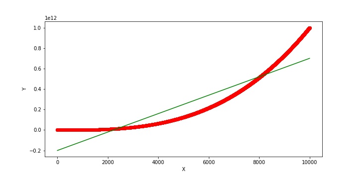
On your graph, the data points are the red line (actually lots and lots of data points and not really a line!). And, the green line is the linear fit. You don’t usually think of Pearson’s correlation as modeling the data but it uses a linear fit. So, the green line is how Pearson’s correlation models your data. You can see that the model doesn’t fit the data adequately. There are systematic (i.e., non-random departures) from the data points. Right there you know that Pearson’s correlation is invalid for these data.
Your data has an upward trend. That is, as X increases, Y also increases. And Pearson’s partially captures that trend. Hence, the positive slope for the green line and the positive correlation you calculated. But, it’s not perfect. You need a better model! In terms of correlation, the graph displays a monotonic relationship and Spearman’s correlation would be a good candidate. Or, you could use regression analysis and include a polynomial to model the curvature. Either of these methods will produce a better fit and more accurate results!
I hope that helps!
Hi jim,
i am ronak from india.
how are you?…hoping corona has not troubled you much.
you have simplified concept very well. you are doing amazing job ,great work. i have one doubt and want to clarify it.
Question : whenever we talk correlation coefficient we talk in terms of linear relationship. but i have calculated
correlation coefficient for relationship Y vs X^3.
X variable : 1 to 10000
Y = X^3
and correlation coefficient is coming around 0.9165. it is strange even relationship is not linear still it is giving me very high correlation coefficient.
Hi Ronak,
I’m doing well here. Just hunkering down like everyone else! I hope you’re doing well too! 🙂
For your data, I’d recommend graphing them in a scatterplot and fit a linear trend line. You can do that in Excel. If your data follow an S-shaped cubic relationship, it is still possible to get a relatively strong correlation. You’ll be able to see how that happens in the scatterplot with trend line. There’s an overall trend to the data that your line follows, but it does hug the curves. However, if you fit a model with a cubic term to fit the curves, you’ll get a better model.
So, let’s switch from a correlation to R-squared. Your correlation of 0.9165 corresponds to an R-squared of 0.84. I’m literally squaring your correlation coefficient to get the R-squared value. Now, fit a regression model with the quadratic and cubic terms to fit your data. You’ll find that your R-squared for this model is higher than for the linear model.
In short, the linear correlation is capturing the overall trend in the data but doesn’t fit the data points as well as the model designed for curvilinear data. Your correlation seems good but it doesn’t fully fit the data.
Hi Jim
Do the partial correlation include the continuous (scale) variables all times?
Is it possible to include other types of variables (as nominal or ordinal)?
Regards
Jagar
Hi Jagar,
Pearson correlations are for continuous data that follow a linear relationship. If you have ordinal data or continuous data that follow a monotonic relationship, you can use Spearman’s correlation.
There are correlations specifically for nominal data. I need to write a blog post about those!
if the correlation coefficient is 0.153 what type of correlation is it?
Hi Jim
Do the partial correlation include the continuous (scale) variables all times?
Is it possible to include other types of variables (as nominal or ordinal)?
Regards
Jagar
If my r value when finding correlation between two things is -0.0258 what would that be negative weak correlation or something else?
Hi Dez, your correlation coefficient is essentially zero, which indicates no relationship between the variables. As one variable increases, there is no tendency for the variable to either increase or decrease. There’s just no relationship between them according to your data.
Hello
my coefficient correlation between my independent variables (anger, anxiety, happiness, satisfaction) and a dependent variable(entrepreneurial decision making behavior) is 0.401, 0.303, 0.369, 0.384.
what does this mean? how do i interpret explain this? what’s the relationship?
Hi Faryal,
It means that separately each independent variable (IV) has a positive correlation with the dependent variable (DV). As each IV increases, the DV tends to increase. However, it is a fairly weak correlation. Additionally, these correlations don’t control for confounding variables. You should perform a regression analysis because you have your IVs and DV. Your model will tell how much variability the IVs account for in the DV collectively. And, it will control for the other variables in the model, which can help reduce omitted variable bias.
The information in this post should help you interpret your correlation coefficients. Just read through it carefully.
Hello there,
If one were to find out the correlation between the average grade and a variable, could this coefficient be used?
Thanks!
Hi Lili,
If you mean something like an average grade per student and the other variable is something like the number of hours each student studies, yes, that’s fine. You just need to be sure that the average grade applies to one person and that the other variable applies to the same person. You can’t use a class average and then the other variable is for individuals.
I’m helping a friend working on a paper and don’t have the variables. The question centers around the nature of Criterion Referenced Tests, in general, i.e. correlations of CRT vs. Norm Referenced Tests. As you know, Norm Referenced compares students to each other across a wide population. In this paper, the student is creating a teacher made CRT. It is measuring proficiency of students of more similar abilities and smaller population to criteria and not to each other. I suspect, in general, the CRT doesn’t distinguish as well between students with similar abilities and knowledge. Therefore, the reliability coefficients, in general, are less reliable. How does this effect high or low correlations?
high or lower correlation on a CRT proficiency test good or bad?
Hi Raymond, I’d have to know more about the variables to have an idea about what the correlation means.
Hello,
I have zero statistics experience but I want to spice up a paper that I’m writing with some quants. And so learned the basics about Pearson correlation on SPSS and I plugged in my data. Now, here’s where it gets “interesting.” Two sets of numbers show up: One on the Pearson Correlation row and below that is the Sig. (2-tailed) row.
I’m too embarrassed to ask folks around me (because I should already know this!). So, let me ask you: which of the row of numbers should I use in my analysis about the correlations between two variables? For example, my independent variable correlates with the dependent variable at -.002 on the first (Pearson Correlation) row. But below that is the Sig. (2-tailed) .995. What does that mean? And is it necessary to have both numbers?
I would really appreciate your response … and will acknowledge you (if the paper gets published).
Many thanks from an old-school qualitative researcher struggling in the times of quants! 🙂
Hi Pat,
The one you want to use for a measure of association is the Pearson Correlation. The other value is the p-value. The p-value is for a hypothesis test that determines whether your correlation value is significantly different from zero (no correlation).
If we take your -0.002 correlation and it’s p-value (0.995), we’d interpret that as meaning that your sample contains insufficient evidence to conclude that the population correlation is not zero. Given how close the correlation is to zero, that’s not surprising! Zero correlation indicates there is no tendency for one variable to either increase or decrease as the other variable increases. In other words, there is no relationship between them.
I hope that helps!
Hi Jim,
Thank you for the good explanation.
I am looking for the source or an article that states that most correlations regarding human behaviour are around .6. What source did you use?
Kind regards,
Amy
Hi Jim,
This is an informative article and I agree with most of what is said, but this particular sentence might be misleading to readers: “R-squared is a primary measure of how well a regression model fits the data.”. R-squared is in fact based on the assumption that the regression model fits the data to a reasonable extent therefore it cannot also simultaneously be a measure of the goodness of said fit.
The rest of the claims regarding R-squared I completely agree with.
Cheers,
Georgi
Hi Georgi,
Yes, I make that exact point repeatedly throughout multiple blog posts, particularly my post about R-squared.
Additionally, R-squared is a goodness-of-fit measure, so it is not misleading to say that it measures how well the model fits the data. Yes, it is not a 100% informative measure by itself. You’d also need to assess residual plots in conjunction with the R-squared. Again, that’s a point that I make repeatedly.
I don’t mind disagreements, but I do ask that before disagreeing, you read what I write about a topic to understand what I’m saying. In this case, you would’ve found in my various topics about R-squared and residual plots that we’re saying the same thing.
Thank you very much!
Hi Jim, I have a question for you – and thank you in advance for responding to it 🙂
Set A has the correlation coefficient of .25 and Set B has the correlation of .9, Which set has the steeper trend line? A or B?
Hi Amy,
Set B has a stronger relationship. However, that’s not quite equivalent to saying it has a steeper trend line. It means the data points fall closer to the line.
If you look at the examples in this post, you’ll notice that all the positive correlations have roughly equal slopes despite having different correlations. Instead, you see the points moving closer to the line as the strength of the relationship increases. The only exception is that a correlation of zero has a slope of zero.
The point being that you can’t tell from the correlation alone which trend line is steeper. However, the relationship in Set B is much stronger than the relationship in Set A.
Thank you ?. Now I understand.
hi, I’m a little confused.
What does it indicating, If there is positive correlation, but negative coefficient from multiple regression outcome? in this situation, how to interpret? the relationship is negative or positive?
Hi JN,
This is likely a case of omitted variable bias. A pairwise correlation involves just two variables. Multiple regression analysis involves three variables at a minimum (2 IVs and a DV). Correlation doesn’t control for other variables while regression analysis controls for the other variables in the model. That can explain the different relationships. Omitted variable bias occurs under specific conditions. Click the link to read about when it occurs. I include an example where I first look at a pair of variables and then three variables and shows how that changes the results, similar to your example.
Hi Jim,
I have 4 objective in my research and when I did the correlation between first one and others the result is:
ob1 with ob2 is (0.87) – ob1 with ob3 is (0.84) – ob1 with ob4 is ( 0.83). My question is what is that meaning and can I do Correlation Coefficient with all of them in one time.
Hi, Mr Jim
Which best describes the correlation coefficient for r=.08?
Hi Jolette,
I’d say that is an extremely weak correlation. I’d want to see its p-value. If it’s not significant, then you can’t conclude that the correlation is different from zero (no correlation). Is there something else particular you want to know about it?
Correlation result between Vul and FCV
t = 3.4535, df = 306, p-value = 0.0006314
alternative hypothesis: true correlation is not equal to 0
95 percent confidence interval:
0.08373962 0.29897226
sample estimates:
cor
0.1936854
What does this mean?
Hi Lakshmi,
It means that your correlation coefficient is ~0.19. That’s the sample estimate. However, because you’re working with a sample, there’s always sample error and so the population correlation is probably not exactly equal to the sample value. The confidence interval indications that you can be 95% confident that the true population correlation falls between ~0.08 and 0.30. The p-value is less than any common significance level. Consequently, you can reject the null hypothesis that the population correlation equals zero and conclude that it does not equal zero. In other words, the correlation you see in the sample is likely to exist in the population.
A correlation of 0.19 is a fairly weak relationship. However, even though it is weak, you have enough evidence to conclude that it exists in the population.
I hope that helps!
Hi Jim
Thank you for your support.
I have a question that is.
Testing criteria for Validity by Pearson correlation,
r table determine by formula DF=N-2
– If it is Valid the correlation value less that Pearson correlation value. (Pearson correlation > r table )
– if it is Invalid the correlation value greater that Pearson correlation value. (Pearson correlation < r table )
I got the above information on SPSS tutorial Video about Pearson correlation.
but I didn't get on other literature please
can you recommend me some literature that refers about this?
or can you clarify more about how to check Validity by Pearson correlation?
HI JIM i am zia from pakistan i wanna finding correlation of two factoer i have find 144.6 of 66.93 thats is postive relation?
Hi Zia, I’m sorry but I’m not clear about what you’re asking. Correlation coefficients range between -1 and +1, so those two values are not correlation coefficients. Are they regression coefficients?
Dear Sir,
Warmest greetings.
My name is Norshidah Nordin and I am very grateful if you could provide me some answers to the following questions.
1) Can I used two different set of samples (for e.g. students academic performance (CGPA) as dependent variable and teacher’s self efficacy as dependent variable) to run on a Pearson correlation analysis. If yes, could you elaborate on this aspect.
2) what is the minimum sample size to use in multiple regression analysis.
Thank You
Hi Norshidah,
For correlations, you need to have multiple measurements on the same item or person. In your scenario, it sounds like you’re taking different measurements on different people. Pearson’s correlation would not be appropriate.
The minimum sample size for multiple regression depends on the number of terms you need to include in your model. Read my post about overfitting regression models, which occurs when you have too few observations for the number of model terms.
I hope this helps!
Greetings sir, question…. Can you do an accurate regression with a Pearson’s correlation coefficient of 0.10? Why or Why not?
Hi Monique,
It is possible. First, you should determine whether that correlation is statistically significant. You’re seeing a correlation in your sample, but you want to be confident that is also exists in the large population you’re studying. There’s a possibility that the correlation only exists in your sample by random chance and does not exist in the population–particularly with such a low coefficient. So, check the p-value for the coefficient. If it’s significant, you have reason to proceed with the regression analysis. Additionally, graph your data. Pearson’s only is for linear relationships. Perhaps your coefficient is low because the relationship is curved?
You can fit the regression model to your data. A correlation of 0.10 equates to an R-squared of only 0.01, which is very low. Perhaps adding more independent variables will increase the R-squared. Even if the r-squared stays very low, if your independent variable is significant, you’re still learning something from your regression model. To understand what you can learn in this situation, read my post about regression models with significant variables and a low R-squared values.
So, it is possible to do a valid regression and learn useful information even when the correlation is so low. But, you need to check for significance along the way.
Hello Jim, first and foremost thank you for giving us a comprehensive information regarding this! This totally help me. But I have a question; my pearson results showing that there’s a moderate positive relationship between my variables which is Parasocial Interaction and the fans’ purchase intention.
But the thing is, if I look at the answer majority of my participants are mostly answering Neutral regarding purchase intention.
What does this means? could you help me to figure out this T.T thanks you in advance! I’m a student currently doing thesis from Malaysia.
Hi Titania,
Have you graphed your data using a scatterplot? I’d highly recommend that because I think it will probably clarify what your data are telling you. Also, are both of your variables continuous variables? I’m wonder if purchase intention is ordinal if one of the values is Neutral. If that’s the case, you’d need to use Spearman’s Rank Correlation rather than Pearson’s.
Hello Jim ! I have a question . I calculated a correlation coefficient between the scale variables and got 0.36, which is relatively weak since it gives a 0.12 if quared. What does the interpretation of correlation concern ? The sample taken or the type of data measurement ? or anything else?
I hope you got my question. Thank you for your help!!
Hi Aya,
I’m not clear what you’re asking exactly. Please clarify. The correlation measures the strength of the relationship between the two continuous variables, as I explain in this article.
Yes, that it is a weak relationship. If you’re going to include this is a regression analysis, you might want to read my article about interpreting low R-squared values.
I’m not sure what you mean by scale variables. However, if these are Likert scale items, you’ll need to use Spearman’s correlation instead of Pearson’s correlation.
Hi Jim
I am very new to statistics and data analysis. I am doing a quantitative study and my sample size is 200 participants. So far I have only obtained 50 complete responses. . Using G*Power a simple linear regression with a medium effect size, an alpha of .05, and a power level of .80 can I do a data analysis with this small sample.
Hi Egbert,
Please repost your question in the comments section of the appropriate article. It has nothing to do with correlation coefficients. Use the search bar part way down in the right column and search for power. I have a post about power analysis that is a good fit.
Thank you Mr.Jim, it was a great answer for me!?
Take good care~
Hi Mr.Jim,
I am a student from Malaysia.
I have a question to ask Mr.Jim about how to determine the validity (the accurate figure) of the data for analysis purpose base on the table of Pearson’s Correlation Coefficient? Do it has any method?
For example, since the coefficient between one independent variable with the other variable is below 0.7, thus the data valid for analysis purpose.
However, I have read the table there is a figure which more than 0.7. I am not sure about that.
Hope to hearing from Mr.Jim soon. Thank you.
Hi, I hope you’re doing well!
There is no single correlation coefficient value that determines whether it is valid to study. It partly depends on your subject area. I low noise physical process might often have a correlation in the very high 0.9s and 0.8 would be considered unacceptable. However, in a study of human behavior, it’s normal and acceptable to have much lower correlations. For example a correlation of 0.5 might be considered very good. Of course, I’m writing the positive values, but the same applies to negative correlations too.
It also depends on what the purpose of your study. If you’re doing something practical, such as describing the relationship between material composition and strength, there might be very specific requirements about how strong that relationship must be for it to be useful. It’s based on real-world practicalities. On the other hand, if you’re just studying something for the sake of science and expanding knowledge, lower correlations might still be interesting.
So, there’s not single answer. It depends on the subject-area you are studying and the purpose of your study.
I hope that helps!
HI Jim, what could be the implication of my result if I obtained a weak relationship between industry experience and instructional effectiveness? thanks in advance
Hi Irene,
The best way to think of it is to look at the graphs in this article and compare the higher correlation graphs to the lower correlation graphs. In the higher correlation graphs, if you know the value of one variable, you have a more precise prediction of the value of the other variable. Look along the x-axis and pick a value. In the higher correlation graphs, the range of y-values that correspond to your x-value is narrower. That range is relatively wide for lower correlations.
For your example, I’ll assume there is a positive correlation. As industry experience increases, instructional effectiveness also increases. However, because that relationship is weak, the range of instructional effectiveness for any given value of industry experience is relatively wide.
I hope this helps!
if correlation between X and Y is 0.8 .what is the correlation of -X and -Y
Hi Tushar,
If you take all the values of X and multiply them by -1 and do the same for Y, your correlation would still be 0.8.
This is very helpful, thank you Jim!
Hi, My data is continuous – the variables are individual shares volatility and oil prices and they were non-normal. I used Kendall’s Tau and did not rank the data or alter it in any way. Can my results be trusted?
Hi Lorraine,
Kendall’s Tau is a correlation coefficient for ranked data. Even though you might not have ranked your data, your statistical software must have created the ranks behind the scenes.
Typically, you’ll use Pearson’s correlation when you have continuous data that have a straight line relationship. If your data are ordinal, ranked, or do not have a straight line relationship, using something other than Pearson’s correlation is necessary.
You mention that your data are nonnormal. Technically, you want to graph your data and look at the shape of the relationship rather than assessing the distribution for each variable. Although, nonnormality can make a linear relationship less likely. So, graph your data on a scatterplot and see what it looks like. If it is close to a straight line, you should probably use Pearson’s correlation. If it’s not a straight line relationship, you might need to use something like Kendall’s Tau or Spearman’s rho coefficient, both of which are based on ranked data. While Spearman’s rho is more commonly used, Kendall’s Tau has preferable statistical properties.
Hi, Jim.
If correlations between continuous variables can be measured using Pearson’s, how is correlation between categorical variables measured?
Thank you.
Hi Yohan,
There are several possible methods, although unlike with continuous data, there doesn’t seem to be a consensus best approach.
But, first off, if you want to determine whether the relationship between categorical variables is statistically significant, use the chi-square test of independence. This test determines whether the relationship between categorical variables is significant, but it does not tell you the degree of correlation.
For the correlation values themselves, there are different methods, such as Goodman and Kruskal’s lambda, Cramér’s V (or phi) for categorical variables with more than 2 levels, and the Phi coefficient for binary data. There are several others that are available as well. Offhand I don’t know the relative pros and cons of each methodology. Perhaps that would be a good post for the future!
Thanks, great explanations.
Hi Jim,
In a multi-variable regression model, is there a method for determining where two predictor variables are correlated in their impact on the outcome variable?
If so, then how is this type of scenario determined, and handled?
Thanks,
Curt
Hi Curt,
When predictors are correlated, it’s known as multicollinearity. This condition reduces the precision of the coefficient estimates. I’ve written a post about it: Multicollinearity: Detection, Problems, and Solutions. That post should answer all your questions!
Hi Jim: Great explanations. One quick thing, because the probability distribution is asymptotic, there is no p=.000. The probability can never be zero. I see students reporting that or p<.000 all of the time. The actual number may be p <.00000001, so setting a level of p < .001 is usually the best thing to do and seems like journal editors want that when reporting data. Your thoughts?
Hi Susan, yes, you’re correct about that. You can’t have a p-value that equals zero. Sometimes software will round down when it’s a very small value. The underlying issue is that no matter how large the difference between your sample value and the null hypothesis value, there is a non-zero probability that you’d obtain the observed results when the null is true.
As for whether it’s a good practice, it probably is one because it makes it explicit. For the p-value that the software displays in this post of 0.000, that actually indicates that it is p < 0.0005. If it was greater than or equal to that value, the software would have rounded it up to 0.001. But, it must've been less than that value. It makes it a bit more clear that there is a tiny probability rather than a zero probability!
Sir you are love. Such a nice share
Awesome stuff, really helpful
Hi there,
What do you do when you can’t perform randomized controlled experiments, like in the cases of social science or societal wide health issues? Apropos to gun violence in America, there appears to be correlation between the availability of guns in a society and the number of gun deaths in a society, where as the number of guns in the society goes up the number of gun deaths go up. This is true of individual states in the US where gun availability differs, and also in countries where gun availability differs. But, when/how can you come to a determination that lowering the number of guns available in a society could reasonably be said to lower the number of gun deaths in that society.
Thanks!
Hi Patrick,
It is difficult proving causality using observational studies rather than randomized experiments.
In my mind, the following approach can help when you’re trying to use observational studies to show that A causes B.
In observational study, you need to worry about confounding variables because the study is not randomized. These confounding variables can provide alternative explanations for the effect/correlations. If you can include all confounding variables in the analysis, it makes the case stronger because it helps rule out other causes. You must also show that A precedes B. Further, it helps if you can demonstrate the mechanism by which A causes B. That mechanism requires subject-area knowledge beyond just a statistical test.
Those are some ideas that come to my mind after brief reflection. There might well be more and, of course, there will be variations based on the study-area.
I hope this helps!
Dear Jim,
Thank you so much, I am learning a lot of thing from you!
Please, keep doing this great job!
Best regards
PS
You bet, Patrik!
Another question is: should I consider transform my variable before using person correlation, if they do not follow normal distribution or if the two variable do not have a clear liner relationship? What is the implication of that transformation? How to interpret the relationship if used transformed variable (let“s say log)?
Because the data need to follow the bivariate normal distribution to use the hypothesis test, I’d assume the transformation process would be more complex than transforming each variable individually. However, I’m not sure about this.
However, if you just want to make a straight line for the correlation to assess, I’d be careful about that too. The correlation of the transformed data would not apply to the untransformed data. One solution would be to use Spearman’s rank order correlation. Another would be to use regression analysis. In regression analysis, you can fit curves, use transformations, etc., and the assumption is that the residual follow a normal distribution (along with some other assumptions) is easy to check.
If you’re not sure that your data fit the assumptions for Pearson’s correlation, consider using regression instead. There are more tools there for you to use.
Hi Jim,
I am always here following your posts.
I would like if you could clarify something to me, please!
What is the assumptions for person correlation that must hold true, in order to apply correlation coefficient?
I have read something on the internet, but there is many confusion. Some people are saying that the dependent variable (if have) must be normally distributed, other saying both (dependent and independent) must be following normal distribution. Therefore, I dont know which one I should follow. I would appreciate a lot your kind contribution. This is something that I am using for my paper.
Thank you in advance!
Hi Patrik,
I’m so glad to see that you’re hear reading and learning!
This issue turns out to be a bit complicated!
The assumption is actually that the two variables follow a bivariate normal distribution. I won’t go into that here in much detail, but a bivariate normal distribution is more complex than just each variable following a normal distribution. In a nutshell, if you plot data that follow a bivariate normal distribution on a scatterplot, it’ll appear as an elliptical shape.
In terms of the the correlation coefficient, that simply describes the relationship between the data. It is what it is and the data don’t need to follow a bivariate normal distribution as long as you are assessing a linear relationship.
On the other hand, the hypothesis test of Pearson’s correlation coefficient does assume that the data follow a bivariate normal distribution. If you want to test whether the coefficient equals zero, then you need to satisfy this assumption. However, one thing I’m not sure about is whether the test is robust to departures from normality. For example, a 1-sample t-test assumes normality, but with a large enough sample size you don’t need to satisfy this assumption. I’m not sure if a similar sample size requirement applies to this particular test.
I hope this clarifies this issue a bit!
Hello,
thanks for the good explanation.
Do variables have to be normally distributed to be analyzed in a Pearson’s correlation?
Thanks,
Moritz
Hi Moritz,
No, the variables do not need to follow a normal distribution to use Pearson’s correlation. However, you do need to graph the data on a scatterplot to be sure that the relationship between the variables is linear rather than curved. For curved relationships, consider using Spearman’s rank correlation.
Pearson’s correlation measures only linear relationships. But regression can be performed with nonlinear functions, and the software will calculate a value of R^2. What is the meaning of an R^2 value when it accompanies a nonlinear regression?
Hi Jerry, you raise an important point. R^2 is actually not a valid measure in nonlinear models. To read about why, read my post about R-squared in nonlinear models. In that post, I write about why it’s problematic that many statistical software packages do calculate R-squared values for nonlinear regression. Instead, you should use a different goodness-of-fit measure, such as the standard error of the regression.
Hi, fantastic blog, very helpful. I was hoping I could ask a question?
You talk about correlation coefficients but I was wondering if you have a section that talks about the slope of an association? For example, am I right in thinking that the slope is equal to the standardized coefficient from a regression?
I refer to the paper of Cameron et al., (The Aging of Elastic and Muscular
Arteries. Diabetes Care 26:2133–2138, 2003) where in table 3 they report a correlation and a slope. Is the correlation the r value and the slope the beta value?
Many thanks,
Matt
Hi Matt,
Thanks and I’m glad you found the blog to be helpful!
Typically, you’d use regression analysis to obtain the slope and correlation to obtain the correlation coefficient. These statistics represent fairly different types of information. The correlation coefficient (r) is more closely related to R^2 in simple regression analysis because both statistics measure how close the data points fall to a line. Not surprisingly if you square r, you obtain R^2.
However, you can use r to calculate the slope coefficient. To do that, you’ll need some other information–the standard deviation of the X variable and the standard deviation of the Y variable.
The formula for the slope in simple regression = r(standard deviation of Y/standard deviation of X).
For more information, read my post about slope coefficients and their p-values in regression analysis. I think that will answer a lot of your questions.
I hope this helps!
Hi,
Nice post ! About pitfalls regarding correlation’s interpretation, here’s a funny database:
http://www.tylervigen.com/spurious-correlations
And a nice and poetic illustration of the concept of correlation:
https://www.youtube.com/watch?v=VFjaBh12C6s&t=0s&index=4&list=PLCkLQOAPOtT1xqDNK8m6IC1bgYCxGZJb_
Have a nice day
Hi Pascal,
Thanks for sharing those links! It always fun finding strange correlations like that.
The link for spurious correlations illustrates an important point. Many of those funny correlations are for time series data where both variables have a long-term trend. If you have two variables that you measure over time and they both have long term trends, those two variables will have a strong correlation even if there is no real connection between them!
Hi.
“In statistics, you typically need to perform a randomized, controlled experiment to determine that a relationship is causal rather than merely correlation.”
Would you please provide an example where you can reasonably conclude that x causes y? And how do you know there isn’t a z that you didn’t control for?
Thanks.
Hi Jerome,
That’s a great question. The trick is that when you perform an experiment, you should randomly assign subjects to treatment and control groups. This process randomly distributes any other characteristics that are related to the outcome variable (y). Suppose there is a z that is correlated to the outcome. That z gets randomly distributed between the treatment and control groups. The end result is that z should exist in all groups in roughly equal amounts. This equal distribution should occur even if you don’t know what z is. And, that’s the beautiful thing about random assignment. You don’t need to know everything that can affect the outcome, but random assignment still takes care of it all.
Consequently, if there is a relationship between a treatment and the outcome, you can be pretty certain that the treatment causes the changes in the outcome because all other correlation-only relationships should’ve been randomized away.
I’ll be writing about random assignment in the near future. And, I’ve written about the effectiveness of flu shots, which is based on randomized controlled trials.
I hope this helps!