What are Interaction Effects?
An interaction effect occurs when the effect of one variable depends on the value of another variable. Interaction effects are common in regression models, ANOVA, and designed experiments. In this post, I explain interaction effects, the interaction effect test, how to interpret interaction models, and describe the problems you can face if you don’t include them in your model.
In any study, whether it’s a taste test or a manufacturing process, many variables can affect the outcome. Changing these variables can affect the outcome directly. For instance, changing the food condiment in a taste test can affect the overall enjoyment. In this manner, analysts use models to assess the relationship between each independent variable and the dependent variable. This kind of an effect is called a main effect. While main effects are relatively straightforward, it can be a mistake to assess only main effects.
In more complex study areas, the independent variables might interact with each other. Interaction effects indicate that a third variable influences the relationship between an independent and dependent variable. In this situation, statisticians say that these variables interact because the relationship between an independent and dependent variable changes depending on the value of a third variable. This type of effect makes the model more complex, but if the real world behaves this way, it is critical to incorporate it in your model. For example, the relationship between condiments and enjoyment probably depends on the type of food—as we’ll see in this post!
Example of Interaction Effects with Categorical Independent Variables
I think of interaction effects as an “it depends” effect. You’ll see why! Let’s start with an intuitive example to help you understand these effects in an interaction model conceptually.
Imagine that we are conducting a taste test to determine which food condiment produces the highest enjoyment. We’ll perform a two-way ANOVA where our dependent variable is Enjoyment. Our two independent variables are both categorical variables: Food and Condiment.
Our ANOVA model with the interaction term is:
Satisfaction = Food Condiment Food*Condiment
To keep things simple, we’ll include only two foods (ice cream and hot dogs) and two condiments (chocolate sauce and mustard) in our analysis.
 Given the specifics of the example, an interaction effect would not be surprising. If someone asks you, “Do you prefer ketchup or chocolate sauce on your food?” Undoubtedly, you will respond, “It depends on the type of food!” That’s the “it depends” nature of an interaction effect. You cannot answer the question without knowing more information about the other variable in the interaction term—which is the type of food in our example!
That’s the concept. Now, I’ll show you how to include an interaction term in your model and how to interpret the results.
How to Interpret Interaction Effects
 Let’s perform our analysis. All statistical software allow you to add interaction terms in a model. Download the CSV data file to try it yourself: Interactions_Categorical.
Use the p-value for an interaction term to test its significance. In the output below, the circled p-value tells us that the interaction effect test (Food*Condiment) is statistically significant. Consequently, we know that the satisfaction you derive from the condiment depends on the type of food.


But how do we interpret the interaction in a model and truly understand what the data are saying? The best way to understand these effects is with a special type of line chart—an interaction plot. This type of plot displays the fitted values of the dependent variable on the y-axis while the x-axis shows the values of the first independent variable. Meanwhile, the various lines represent values of the second independent variable.
On an interaction plot, parallel lines indicate that there is no interaction effect while different slopes suggest that one might be present. Below is the plot for Food*Condiment.

The crossed lines on the graph suggest that there is an interaction effect, which the significant p-value for the Food*Condiment term confirms. The graph shows that enjoyment levels are higher for chocolate sauce when the food is ice cream. Conversely, satisfaction levels are higher for mustard when the food is a hot dog. If you put mustard on ice cream or chocolate sauce on hot dogs, you won’t be happy!
Which condiment is best? It depends on the type of food, and we’ve used statistics to demonstrate this effect.
Overlooking Interaction Effects is Dangerous!
When you have statistically significant interaction effects, you can’t interpret the main effects without considering the interactions. In the previous example, you can’t answer the question about which condiment is better without knowing the type of food. Again, “it depends.”
Suppose we want to maximize satisfaction by choosing the best food and the best condiment. However, imagine that we forgot to include the interaction effect and assessed only the main effects. We’ll make our decision based on the main effects plots below.

Based on these plots, we’d choose hot dogs with chocolate sauce because they each produce higher enjoyment. That’s not a good choice despite what the main effects show! When you have statistically significant interactions, you cannot interpret the main effect without considering the interaction effects.
Given the intentionally intuitive nature of our silly example, the consequence of disregarding the interaction effect is evident at a passing glance. However, that is not always the case, as you’ll see in the next example.
Example of an Interaction Effect with Continuous Independent Variables
For our next example, we’ll assess continuous independent variables in a regression model for a manufacturing process. The independent variables (processing time, temperature, and pressure) affect the dependent variable (product strength). Here’s the CSV data file if you want to try it yourself: Interactions_Continuous. To learn how to recreate the continuous interaction plot using Excel, download this Excel file: Continuous Interaction Excel.
In the interaction model, I’ll include temperature*pressure as an interaction effect. The results are below.


As you can see, the interaction effect test is statistically significant. But how do you interpret the interaction coefficient in the regression equation? You could try entering values into the regression equation and piece things together. However, it is much easier to use interaction plots!
Related post: How to Interpret Regression Coefficients and Their P-values for Main Effects

In the graph above, the variables are continuous rather than categorical. To produce the plot, the statistical software chooses a high value and a low value for pressure and enters them into the equation along with the range of values for temperature.
As you can see, the relationship between temperature and strength changes direction based on the pressure. For high pressures, there is a positive relationship between temperature and strength while for low pressures it is a negative relationship. By including the interaction term in the model, you can capture relationships that change based on the value of another variable.
If you want to maximize product strength and someone asks you if the process should use a high or low temperature, you’d have to respond, “It depends.” In this case, it depends on the pressure. You cannot answer the question about temperature without knowing the pressure value.
Important Considerations for Interaction Effects
While the plots help you interpret the interaction effects, use a hypothesis test to determine whether the effect is statistically significant. Plots can display non-parallel lines that represent random sampling error rather than an actual effect. P-values and hypothesis tests help you sort out the real effects from the noise.
The examples in this post are two-way interactions because there are two independent variables in each term (Food*Condiment and Temperature*Pressure). It’s equally valid to interpret these effects in two ways. For example, the relationship between:
- Satisfaction and Condiment depends on Food.
- Satisfaction and Food depends on Condiment.
You can have higher-order interactions. For example, a three-way interaction has three variables in the term, such as Food*Condiment*X. In this case, the relationship between Satisfaction and Condiment depends on both Food and X. However, this type of effect is challenging to interpret. In practice, analysts use them infrequently. However, in some models, they might be necessary to provide an adequate fit.
Finally, when an interaction effect test is statistically significant, do not attempt to interpret the main effects without considering the interaction effects. As the examples show, you will draw the wrong the conclusions!
If you’re learning regression and like the approach I use in my blog, check out my Intuitive Guide to Regression Analysis book! You can find it on Amazon and other retailers.

Share this:

Reader Interactions
Comments
Comments and Questions

Hi Jim, great examples and very helpful, especially to my students! This is maybe an obvious question, but I find myself overthinking it and not finding a clear answer elsewhere online, so I wanted to ask – I’m using some interaction terms in SEM/path analysis (both variables are continuous, so it makes more sense than a multi-group analysis, and all variables are observed, b/c I know AMOS won’t do interaction terms of latent variables). I’ve created the interaction terms using centering, but conceptually, it still seems like it would make sense to correlate the error of the centered interaction term with the errors of each of its component variables? But is this correct? So in other words, if I am testing an interaction between depression and age and their joint influence on marital satisfaction (not my actual variables, making these up), and I then create an interaction term by multiplying centered versions of depression and age and specifying a path from that interaction term to marital satisfaction, as well as from uncentered depression to MS and uncentered age to MS, should I also correlate the error of the interaction term with the errors of depression and age? Or is that inappropriate once I’ve centered the variables to create the interaction term? Thanks!
Thank you for your blog. Should I remove a non-significant interaction term between row and column factors while doing a two-way ANOVA analysis and only keep the row and column main effects?
Hi Dave,
Yes, that’s generally the standard approach. An exception would be if you have strong theoretical reasons or previous research that suggests that the interaction effect exists despite the non-significant results.
Hi Jim,
I liked your blog about interactions. I am working with the interaction of two dummy variables and want to interpret its results. Can you please guide me how to do it?
Hi Rajni
In this post, pay particular attention to the mustard and chocolate sauce example. Those are two dummy variables and I work through the interpretation of their interaction effect.
I think part of the answer also lies in the standard error. I was also scratching my head over one of the main effects becoming insignificant (while the interaction was also insignificant), but then I saw the standard error had almost doubled.
That might be due to multicollinearity. Fitting an interaction term increases that. Try centering the variables to see if that helps. Read my post about multicollinearity for more details about this method!
Dear Jim,
Many thanks for your posts. I have a question regarding my results. The regression analysis shows that the coefficient of the interaction term is statistically significant. However, when I plot the lines, the graph shows no interaction effect. How should I interpret my result? Should I rely on the regression result or the graph?
Thank you
Saltanat
Hi Saltanat,
Typically, you’d expect to see either crossing lines or at least obviously non-parallel lines when you have a significant interaction effect. However, there are several possibilities for your case.
Keep in mind that the statistical test for an interaction effect evaluates whether the difference between the slopes is statistically significant. The fact that your interaction effect is significant indicates that the different between the lines is significant whether you see that on the graph or not. Consider, the following possibilities:
Perhaps your model has very high statistical power and can detect trivial differences between the lines. The lines are just barely non-parallel. This might happen if you have a large sample size and/or very low noise data. If this is true, your interaction effect might be statistically significant but probably aren’t practically significant.
Another possibility is the scaling for your graphs might be hiding a difference. That’s probably unlikely but at least worth considering. Perhaps the scaling is too zoomed out?
One thing to do is evaluate the predicted DV values for specific IVs for a model with and without the interaction effect. Do those predicted values change much? If they don’t change much, the interaction effect is not practically significant.
I hope that helps!
Good evening Mr. Frost. Can an interaction effect be found if there are only two variables: tslfest and agegp3?
Hi Candy,
Yes, assuming those two variables are independent variables in a model, it’s entirely possible they have an interaction effect. Two is the minimum number of independent variables that can have an interaction effect. I don’t know about those two specific variables, but it is at least possible.
Thanks for the article, really helpful. Just a question that I have in mind, when we run repeated measures two way anova and find out there is an interaction effect. Is it advisable to run one way anova on each factor to find out the simple effects? In my experiment, I’m using ARTool to trasnform ordinal data so that I could use anova on them https://depts.washington.edu/acelab/proj/art/. The tool documentation mentioend about using IV1*IV2 for pairwise comparison. But what if I want to use one way anova provided by the tool as well to find simple effects? Problem is each apporach generate different results 🙂
Hi Omar,
I’ve only taken a quick look at this tool, but it looks like a good one!
In general, when you have significant interaction effects, you don’t want to focus too much on only the main effects. In this context, the main effects can lead you astray! I show an example of that in this blog post. You really need to understand the interaction effects because in some cases they drastically change your understanding of the main effects. For this reason, whenever I’ve had significant interactions and needed to do pairwise comparisons, I’ve always included the interaction in those comparisons as the tool’s documentations suggests. (I’ve never used the tool but the principle should be the same.) Again, comparing main effects might lead you astray.
If you graph the main and interaction effects as I show in this post, you should be able to see whether the interaction effects significantly change your understanding of the model’s results.
I hope that helps!
How about when all of the two main variables that provide the main effect become statistically insignificant only after including the interaction term but were statistically significant before including the interaction term? And two models have similar residual plots.
Hi Elaine,
That can be a tricky situation. The question becomes, which model is better? The one with or without the interaction terms? It sounds like you could justify either model statistically. Here are some tips to consider.
If your IVs are continuous, center them to reduce multicollinearity in the model with interaction effect. Interaction terms jack up multicollinearity, which can reduce the power of the statistical tests. See if either of the main effects become significance after centering the variables and refitting the model. Click the link to learn more about that process.
If that doesn’t provide a clear answer (i.e., the main effects are still not significant), consider the following.
Is the R-squared and other goodness-of-fit measures notably better for one model or the other? While you don’t necessarily want to chase a high R-squared mindlessly, if one model does provide a better fit, that might help you decide.
Graph the interaction effect to see if it is strong. Perhaps it is statistically significant but practically not significant? I show what interaction plots look like in this post. If an interaction effect produces nearly parallel lines, it is fairly weak even if its p-value is significant.
Input values into the two models and see if it produces similar or different predicted values. It’s possible that despite the different forms of the model, they might be fairly equivalent.
Use subject-area knowledge to help you decide. Is the interaction effect theoretically justified? Evaluate other research and use your expertise to determine which model is better.
How do you interpret when one of the two main variables that provide the main effect become statistically insignificant only after including the interaction term but were statistically significant before including the interaction term?
Hi Simba,
When you include an interaction term in a regression model and observe that one of the main effects becomes statistically insignificant, it suggests that the effect of that variable is conditional on the level of the other variable. In other words, the effect of the main variable is not consistent across all levels of the other variable, and its significance is captured by the interaction term. That variable has no effect that is independent of the other variable.
However, there are several cautions about this interpretation. It’s possible that the main effect exists in the population but your regression analysis lacks sufficient power to detect it after including the interaction term. Remember, failing to reject the null hypothesis does not prove that the effect doesn’t exist. You can’t prove a negative. You just don’t have enough evidence so say that it does exist.
Also, you need to use your subject-area knowledge to theoretically evaluate the two models. Does it make more theoretical sense that the main effect or interaction effect exists? Or, perhaps theory suggests they both exist? Answering those questions will help you determine which model is correct. For more information on that topic, read Specifying the Correct Regression Model. Pay particular attention to the theory section near the end.
It’s always a good idea to plot the interaction to visualize and better understand the relationship.
I know that’s not a definitive answer but understanding those results and determining which model is best requires you to assess it theoretically. Also check those residual plots for each one!
it truly is!
This article was SO helpful, thank you!
Hi Hannah! I’m so glad to hear that it helpful! 🙂
Hi Jim,
Thank you for your helpful link.
I have an issue regarding the quadratic and linear terms in a model. I have studied insect population in many places and plants species. I collected insects randomly every week.
So the model (mixed effects) is as follows:
– Fixed factors (place and plant species),
-Sampling date as quadratic and linear terms
– and plant (from which the insects were collected) as a random effect.
My questions are about the interactions:
1- is it enough to include only binary interaction among those effects: place, plant species and date (quadratic and linear effect)?
2- should I consider quadratic and linear terms in three way interaction (place:plant species:date + place:plant species:date^2)?
I appreciate your help.
Hi Mohannas,
It’s possible to go overboard with higher-order interactions. They become very difficult to interpret. However, if they dramatically improve your model’s fit and are theoretically sound, you should consider add three-way interactions.
However, in practice, I’ve never seen a three-way interaction contribution much to the model. That’s not to say it can’t happen. But only add them if they really make sense theoretically and demonstrably improve your model’s fit.
Hello Jim, what happens when we have to deal with a variable that only has a value if another condition is met? Suppose we run a regression and we want to assess the impact of years of marriage, however this only applies to married people. Can we model the the problem the following way?
y ~ if.married+if.married*years.marriage
If so, how can I interpret the results of this? What does it mean to have a significant main term (if.married) but an insignificant interaction term? If the interaction is insignificant, but the main term is significant, can we just maintain the main term?
Thank you
Hi Jim,
Thank you for your help!
Honestly I didn’t fully understand the part of using post hoc tests.
If I add a categorical variable, with several levels, in a regression (I use R), the output already gives me the p-values, and coefficients, for each level, compared with the reference level. After that, I would run an ANOVA between a model with, and a model without the variable, to test if, overall, the categorical variable is significant or not. But, I got the idea that, what you are sugesting is a test to evaluate the differences among each combination of levels, instead of just the reference (output of a regression). Is that correct?
Hi Isa,
Read my post that I link to and learn about post hoc tests and the need to control the familywise error rate. Yes, you can get the p-values for the difference but with multiple groups there’s an increasing chance of a false positive (despite significant p-values).
There are different ways to assess the mean differences. One is the regression coefficients as you mention, which compares the means to the baseline level. Another is to compare each group’s mean to the other groups means to determine which groups are significantly different from each other. Because you were mentioning creating groups based on all the possible combinations, the all pairwise approach makes more sense than comparing to a baseline level.
But, either way, you should control the familywise error rate. Read my post for information about why that is so important. In particular, you described creating multiple groups for all the combinations and that’s when the familywise error rate really starts to grow!
Hello Jim,
Thanks for your article!
I have a question regarding interactions with binary variables. Considering the example you showed (Food+Condiment) is there any advantage in considering an interaction instead of modelling all possible combinations as a categorical variable?
My suggestion is: instead of doing Food*Condiment, we would create a categorical variable with the following levels: HotDog+Mustard; HotDog+Chocolate; IceCream+Chocolate; IceCream+Mustard. The results would show the difference between that certain level and the reference level. In my opinion this “all levels” approach seems easier to understand but is it correct?
Of course that for categorical variables with several levels (for example, several types of food and several condiments) this solution would be impractical, so I am just talking about two binary variables.
Hi Isa,
Conceptually, you’re correct that you could include in the model the groups based on the combinations of categorical levels. However, there are practical drawbacks for using that approach by itself. That method would require more observations because you need minimum number of observations per group. Additionally, because you’re comparing multiple means, you’d need to use a post hoc multiple comparison method that controls the familywise error rate, which reduces statistical power.
By including an interaction term, you’re directly testing the idea that the relationship between one IV and the DV depends on the value of another IV. You kind of get that with the group approach, but you’re not directly testing the interaction effect. Also, by including the interaction term rather than the groups, you don’t have the sample size problem associated with including more groups nor do you have the need for controlling the familywise error rate. Finally, using interaction plots (or group means displayed in a table), the results are no harder to interpret than using your method.
In practice, I’ve seen both methods used together. Statisticians will often include the interaction term and see if it is significant. If it is and they need to know if the differences between those group means are statistically significant, they can then perform the pairwise multiple comparisons on them. But usually it is worthwhile knowing whether the interaction term is significant, and then possibly determining whether any of the differences between group means are significant.
I’d see the two methods as complementary, but usually starting with the interaction term. I hope that helps!
Hi Jim!
Lots Thank you for explaining these concepts.
I have a question about interaction effect tests.
In my study, I had two groups: a smokers’ group with three categories (including heavy , medium, and light smoking) and a non-smokers’ group (as control )
to evaluate the interaction effect of smoking on the depednent contanous variable (platelet count).
What is the best statistical test that can be applied to determine the effect of smoking on platelet count? What is the best statistical test that can be applied to determine the relationship between smoking and platelet count?
Hi Zaid,
To have an interaction effect, you must have at least two independent variables (IV). Then you can say that the relationship between IV1 and the dependent variable (DV) depends on the value of IV2.
It appears like you only have one IV (smoking level) and you have four levels of that IV (non, light, medium, heavy). You can use one-way ANOVA to find the main effect of smoking on platelet count. That test will tell you if the differences between the groups mean platelet count are statistically significant. Just be aware that is a main effect and not an interaction effect.
Dear Jim, I have an important question on a matter I have to understand for a piece of research I’m conducting myself. You said enjoyment might depend on the Food*Condiment interaction, ok. What I don’t get is a point at a deeper level. Let’s suppose you want to do a repeated measure anova, because the same subject eats different types of foods with different condiments (which is the design of my own research) Let’s assume Food has three levels: sandwiches, pasta and meet and Condiment has two: ketchup and mayonnaise. The interaction might mean two things, among others, that is:
1) WITHIN the “sandwich” level, people prefer it with mayonnaise (higher enjoyment rate for mayonnaise) and not with ketchup. In this case, mayonnaise would show enjoyment rates which are higher in a statistical relevant way than ketchup WITHIN one of the levels of the other factor.
OR:
2) WITHIN “ketchup” level, people prefer to eat ketchup with pasta than with meet. In this other case, the comparison of the enjoyment means from the subjects is between food types and not condiment types.
I am stuck in this point, because the two things are different.
Thank you so much,
Vittorio
Hi Jim, I gain lot of guidance from your discussions on statistics. I am stuck in a concept of multiple regression. If you can guide me it will be a great help. Following is my concept of background working of multiple regression: When we have two independent variables, first, we get residuals of both independent variables by regressing both variables on each other. Then we perform simple regression using residuals of both independent variables against the dependent variable, separately. This step gives us one beta for residual of each variable which is essentially considered as beta of each independent variable in multiple regression. Is this concept true? If so, I can understand that residual of one independent variable is necessary to obtain in order to break the multicollinearity between both independent variables. However, is it fair to get and use residual of second independent variable as well? I tried my best to put question in right way. If you need me to make it more elaborated, I can give it another try. Your answer will be highly appreciated.
Sajid
Hi Muhammad,
When you have two independent variables, you only fit the model once and that model contains both IVs. Hence, even when you have two IVs, you still obtain only one set of residuals. You don’t fit separate models for each IV.
In the future, try to place you comment/question in a more appropriate post. It makes reading through the comments more relevant for each post. To find a closer match, use the search box near the upper right-hand margin of my website. Thanks!
Thank you very much Jim!
Hi Jim
I am having trouble interpreting my own results of a two-way repeated ANOVA and was wondering if you could help me out.
DV: negative affect
IV:sleep quality (good or bad)
IV:gender
I found a significant main effect of sleep quality and negative affect but no significant main effect of gender and negative affect. However, i did find a significant interaction between sleep quality and gender. What could you conclude from this or how would you interpret these results?
Dear mr. Frost,
I have a question regarding the interpretation of the repeated measures ANOVA. I conduct a part of my study to investigate the best way to identify the maximum voluntary contraction (MVC) in healthy subjects between 2 different protocols to measure the MVC (ref) and 4 different methods of determing the MVC (mean of the mean, mean of maximum, maximum of the mean and maximum of maximum). Therefore, in my analysis, I have 2 values of the 2 different protocols and values of 4 the conditions for each examined muscle.
I conducted in my analysis a repeated measures of ANOVA with a Bonferroni. On 1 particular muscle, the serratus anterior (SA), my results of the “Tests of Within-Subjects Effects” state that I have a significant interaction effect between the 4 conditions and the 2 values of the 2 different. So this means that I either have a difference in values between the 2 protocols but not for each condition i gues??
I got stuck with the interpretation of the interaction effects between this 2 types of factors.
Would it be possible for you to help me interpret the results?
Thank you in advance.
Kind regards,
Symon
Hi Jim!
Thank you so much for the quick reply.
When you say increasing the sample size by 10, is that per group or overall? E.g. if I have 20 participants and want to add the sex interaction term, if I have 10 males and 10 females, do I increase the sample size to 30 or 40?
Thank you!
Eva
Hi Eva,
You’re very welcome!
Ah, I’m glad you asked that follow-up question. The guideline for a minimum of 10 observations is for continuous independent variables. It didn’t click with me that gender is, of course, categorical. Unfortunately, it’s a bit more complicated for categorical variables because it depends on the number of groups and how they’re split between the groups. Most requirements for categorical variables assume an even split. I’m forgetting some of the specific guidelines for categorical variables, but I’d guestimate that you’d need an additional 20 observations to add the gender variable with half men (10)/half women (10). If you have unequal group sizes, you’d ensure that the smaller group exceeds the threshold.
In the other post I recommended, I include a reference that discusses this in more detail. I don’t have it on hand, but it might provide additional information about it. Also, given the complexity of your design, I’d be sure to run it by your statisticians to be sure.
Finally, these guidelines are for the minimums. And you’d rather not be right at the minimums if at all possible!
Hi Jim!
Thank you for the straightforward blog posts explaining these concepts.
I have a question about interaction tests.
I am designing an experiment and deciding on which test to use. The study is essentially a biomechanical test pre and post a treatment, so for checking treatment effects on the outputs (which are continuous) I will use a paired t-test. However, I also want to check the effects of sex and menstrual cycle phase. For the menstruating females, they are tested at 3 phases in the cycle. Another group of oral birth control users is also tested at 3 times across the cycle.
Now, one statistician recommended just putting everything in a linear mixed effects model (sex, menstrual cycle phase, birth control). Another one suggested doing the sex comparison separate and testing the change due to treatment between the groups, and then to test menstrual cycle effects comparing change due to fatigue in pairwise tests between phases (1 and 2, 2 and 3 etc) and also comparing between birth control and non birth control users, which ends up being a lot of separate tests.
I was also thinking I could instead test sex effect on the treatment outcome with an ANOVA with interaction (sex x treatment), using the average values for the females (since they are tested 3 times), and then for the menstrual cycle effects check phase x treatment x birth control, or phase x treatment first, and then do a separate test to compare changes due to treatment between birth control users and non birth control users at each phase (or use a linear mixed effects model only for the females).
Regarding the interaction tests, someone raised the issue of increased sample size being needed (https://statmodeling.stat.columbia.edu/2018/03/15/need-16-times-sample-size-estimate-interaction-estimate-main-effect/).
But another person mentioned that if I would do all the separate tests between phases etc then this would be an issue with multiple testing and would need correction. Which I assume would also then require a higher sample size for the same power and effect size, correct?
I am very new to stats so any help is much appreciated, especially explaining pros and cons of these approaches. I am also not sure whether, regardless of the tests for sex and phase, I should do a separate t-test for the primary outcome (pre vs post treatment) first and whether I need to correct p values for this or only for the subsequent tests.
Thank you!
Hi Eva,
As for the general approach, it sounds like you have a fairly complex experiment. My sense is to include as much as you can in a single model and not perform separate tests.
Instead of a paired t-test, use the change in the outcome as your dependent variable. Then include all the various other IVs in the model. This approach improves upon a t-test because you’re still assessing the changes in the outcome, just like a paired t-test, but you’re also accounting for addition sources of variability in the model, which the paired t-test can’t do. If there’s a chance that the treatment works better in women or men, then you should include an interaction term.
Again, I would try to avoid separate tests and build them into the model. Based on the rough view of your experiment that I have, I don’t see the need for separate tests. You can perform the multiple comparison tests as needed to do the adjustments for the multiple tests, but I would have the main tests all be part of the model, and the perform the multiple comparison tests based on the model results.
You definitely need a larger sample size when include interaction terms, or any other type of term (main effect, polynomial for curvature, etc.) I’m not sure that I agree with that link you share that you need 16 times the sample size though. (The author proposes a very specific set of assumptions about relative effect sizes and then generalizes from there. Not all interaction effects will fit his specific assumptions.)
Typically, you should increase your sample size by at least 10 for each additional term. Preferably more than that but 10 is a common guideline. And that’s an increase of 10, NOT 10X! Before collecting data, you should consider all the possible complexities that you might want to include in your model and figure out how many terms that entails. From there, you can develop a sense of the minimum sample size you should obtain.
As I show in this post, if interaction effects are present and you don’t account for them in the model, your results can be misleading! However, you don’t want to add them all willy nilly either.
I write about that in my post about overfitting your model, which includes a reference for sample size guidelines.
I probably didn’t answer all your questions, but it seems like a fairly complex experiment. I think many of the answers will depend on subject-area knowledge that I don’t have. But hopefully some of the tips are helpful!
Hi Jim,
I am currently doing my dissertation and am doing a 3 (price difference: no/low/high, within subjects) X 2 (information level: low/high, between groups) mixed ANOVA to assess the affect of price and information on consumers sustainable shopping decisions. I have significant main effects of both price and information, but the interaction was not significant. When interpreting these results, what does the non-significant interaction tell me about the main effects?
Also is there any other possible reason for the non-significant interaction eg narrow sample type etc?
Thank you!
Hi Jim,
Do you have R code by chance?
Amelia
Hi Jim,
Great!! Thank you for the explanation. Very helpful and informative.
Thank you for the this, great explanation.
My question is, do we rely only on the p-value to indicate significance in interactions?
All thanks
Hi Layan,
In terms of saying whether the interaction is statistically significant or not, yes, you go only by the p-value. However, determining whether to include it or not in your model is a different matter.
You should never reply solely on p-values for fitting your model. They definitely play a role but shouldn’t be the sole decider. For more information about that, read my post, Choosing the Correct Regression Model.
That definitely applies to interaction terms. If you get a significant p-value and the interaction makes theoretical sense, leave it in. However, if it’s significant but runs counter to theory, you should consider excluding it despite the statistical significance. And if the interaction is not significant but theory and/or other studies strongly suggest it should be included, you can include it regardless of the p-value. Just be sure to explain your approach and reasoning in the write-up and include that actual p-value/significance (or not) in your discussion. For example, if it’s not significant but you need to include it for theoretical/other researcher reasons, you’d say something to the effect, “the A*B interaction was not significant in my model, but I’m including it because other research indicates it’s a relevant term.” Then some details about the other research or theory.
I’m not sure if you were asking about only determining significance/nonsignificance or the larger issue of whether to include it in your model, but that’s how to handle both of those questions!
“The other main reason is that when you include the interaction term in the model, it accounts for enough of the variance that the main effect used to account for before you added the interaction, that it is longer significant. If that’s the case, it’s not a problem! It just means that for the main effect in question, that variable’s effect entirely depends on the value of the other variable in the interaction term. None of that variable’s effect is independent of that other variable. That happens sometimes!”
Would this be true if the interaction term was not significant?
Hi Alice,
It can be true. It’s possible that there’s not enough significance to go around, so to speak, leaving both insignificant.
Hi Jim,
Thanks for a great explanation!
What happens if, once you add the interaction term, the main effect is no longer statistically significant, but the interaction term is?
Thank you,
Hania
Hi Hania,
That can happen for a couple of reasons. One, if you have an interaction term that contains two continuous variables, it introduces multicollinearity into the model, which can reduce statistical significance. There’s an easy fix for this problem. Just center your continuous variables, which means you subtract each variable’s mean from all its observed values. I write about this approach and show an example in my post about multicollinearity.
The other main reason is that when you include the interaction term in the model, it accounts for enough of the variance that the main effect used to account for before you added the interaction, that it is longer significant. If that’s the case, it’s not a problem! It just means that for the main effect in question, that variable’s effect entirely depends on the value of the other variable in the interaction term. None of that variable’s effect is independent of that other variable. That happens sometimes!
Thank you Jim, that is really helpful to me!
I am currently on research and in my research I have 3 independent variables (x, y, z) and one dependent variable. after conducting a 3-way ANOVA, I have seen that, all the 3 variables and their interaction are significant. I have no idea what to do next. please help me how to solve this🙏🙏
Dear Jim, thanks for your time, and valuable info . My analysis has result for one of the dimensions impact is statistically insignificant while interaction effect is significant. I was told not right to interpret. Now I see it could be. Can you please send me a source to refer in my thesis? Thx, abd Best Regards
Hi Serap,
My go to reference is Applied Linear Statistical Models by Neter et. al. I haven’t looked to see if it discusses this aspect of interaction effects, but I’d imagine it would in its over 1000 pages!
Yes, when you have significant interaction effects, you need to understand them and incorporate them into your conclusions. Failure to do so can lead you to incorrect conclusions. This is true whether or not your main effects are significant.
Thank you Jim. This is very helpful!
I have one question regarding interaction. Let’s say I have two dichotomous variables A and B. What is the difference between using an interaction term A*B in the model vs. creating a grouping variable that has four levels (A+B+; A+B-; A-B+; A-B-)?
Thanks!
Hi,
In my paper, I have two independent variables (infusion time and amount of lemongrass) which has a significant interaction. I am unsure as to how to explain and support this in words.
Thank you
Hi Jim!!
Thanks for taking your time to answer our questions, I discovered your page today and it’s great!
If you have some time, I would like to ask you about interaction terms in a time series regression, such as an ARDL model. My questions are two.
i) Does an interaction term with two variables, let’s call these X1{t} and X2{t}, need lags in this type of model?
ii) If I have some interaction term like X3{t}=X1{t}*X2{t}, is it necessary to apply a unit root test to check for stationarity, right? In that case, what is the best way to reach it?
Thanks a lot !!!
Hi Jim! Thanks for you post!
How do I report the interaction on the text? Is it correct to say that the codiment has effect on satisfaction only if it interact qith the type of food?
Hi Jim,
How to Automatically judge whether there are interaction terms between independent variables by using a package in R? Is there a way to do this?
As I have 5 categorical independent variables and 4 continuous independent variales. It’s hard for me to check it one by one manually.
Hi Linlin,
I don’t know about R, but various software packages have routines that will try all sort of combinations of variables. However, I do not recommend the use of such automated procedures. That increases your chances for finding chance correlations that are meaningless. Read my post about datamining for more information. Ideally, theory and subject-area knowledge should be guides when specifying your regression model.
Hello Jim,
I got to know about the awesome work you are doing in the statistics field from someone I am following on YouTube and LinkedIn in the Data Analysis and Data Science space(s).
With respect to interactions effects, I have some questions:
(1) should the interaction terms be included in a multiple regression model at all times if they are statistically significant? Or is it the research/study question(s) that should determine their inclusion?
(2) How do you determine the interaction terms to include? For instance, in the second example in this blog of a manufacturing process, I see that you used Pressure and Temperature as the interaction terms.
Finally, I analyzed the data in (2) using Excel. While I obtained the same model output as in your example, the interaction plot I created had parallel lines for high and low pressure respectively, suggesting a lack of interaction. I used this formula
Strength = 0.1210*Temperature*Pressure
to derive fitted/predicted values for the dependent variable along with the high and low values for pressure and the range of values for temperature. Please is there something I did incorrectly?
I wanted to send you an email or post the image here but these have proven difficult.
Hoping to hear from you.
Thank you.
Jefferson
Hi Jefferson,
Sorry about the delay replying! Thanks for writing with the great questions.
In the best case scenario, you add the interaction terms based on theoretical reasons that support there being an interaction effect. You can go “fishing” for a significant interaction term to see if it is significant. But be aware that doing that too much increases your probability of finding chance effects. For more information about that, read my post about data mining. If you do add interaction terms “just to see” and you find a significant one, be sure that it makes logical/theoretical sense.
So, there’s not a hard and fast rule for knowing when to include interaction terms. It’s bit of an art as well as a science. For more details about that aspect, read my post about Model Specification: Choosing the Correct Regression Model. But try to use theory and subject-area knowledge as guides and be sure that the model makes sense in the real-world. You don’t want to be in a situation where the only reason you’re including variables and interactions is just because they’re significant. They have to make sense too.
I’m not sure why your Excel recreation turned out that way. I recreated the graph in Excel myself and got replicated the graph in the post almost exactly. You need to use the entire equation and enter values for all the terms. For the Time variable, I entered the mean time. The Excel version I made is below. Additionally, I’ve added a link to the Excel dataset in the post itself. You can download that and see how I made it.
I hope that helps!
Hi Jim,
I am attempting to explain a three-way interaction.
I examine the effect of X on Y condition on two moderators (W and Z; W and Z are positive values).
I expect that W reduces the negative effect of X on Y; Z strengthens the negative effect of X on Y; and I need to conclude which one has stronger effect on the relationship between X and Y.
Case 1: W and Z are continuous variables, the outcome is:
Y = 0.023 -X(0.941-0.009*W+0.340Z-0.201WZ)
Case 2: W and Z are dummy variables (taking a value of 1 or 0), the outcome is
Y = 0.016 -X(0.967-0.092*1+0.145*1-0.253*1*1) (I replaced W=1 and Z=1)
How I can interpret the three way effect in this case. Could you give me a help?
Thank you
Thank you for your quick response! Really helpful 🙂
Jim,
Thank you so much for your time explaining these concepts! I’m reading medical literature and trying to figure out the difference between a P-interaction and a p-value. This is a very important study with a P-interaction=0.57 so being that it is not <0.05 (statistically significant), I'm thinking P-interaction must be the 3-way interaction rather than the main effects.
Thanks so much!
Becky
Hi Becky,
I don’t know what a P-interaction is? Do you mean a p-value for an interaction term?
P-values for interaction terms work the same way as they do for main effects and I’ve never seen them given a distinct name. When they’re less than your significance level, they indicate that the interaction (or main effect) is statistically significant. More specifically, they’re all testing whether the coefficient for the term (whether it’s for a main effect or interaction effect) equals zero. When your p-value is less than the significance level, the difference between the coefficient and zero is statistically significant. You can reject the null that effect is zero (i.e., rule out no effect). All of that applies to main effects and interaction effects. It’s how you interpret the effect itself that varies.
I hope that helps!
Jim — this is so helpful. I think I get it now. We can imagine a scenario where sleep and study are not correlated. The good students, no matter how much they sleep, still find the time to study. The bad students, no matter how much they sleep, still don’t study much. So sleep hours and study hours are not correlated.
And yet, there can still be an interaction effect between sleep and study. For example, we could imagine that for the students who study a lot, getting extra sleep has a big, positive impact on their GPA. But for the students who study a little, getting extra sleep has only a tiny, positive impact on their GPA.
Thus, there was no correlation between sleep and study, but their interaction was still significant.
Did I get that right?
Hi Max,
Yes, that’s it exactly! There doesn’t need to be a correlation between the IVs for an interaction effect to exist.
Hi Jim, thank you for writing this article!
I was wondering if you could help me with this. I conducted a regression analysis including an interaction between two categorical variables. (Sequel*Book) [yes=1; no=0] on movie performance.
I found a positive significant interaction effect, can I now say that the performance of book on movie performance is based on if it is a sequel or not? And thus suggest that if sequel = 1 this positively affects performance?
Thank you!
Hi Emily,
Yes, if you have that type of interaction and it is statistically significant, you can say that the relationship between Book (Yes/No) and Movie Performance depends on whether it’s a sequel. Using an interaction plot should help bring the relationships to life. From what you write, it sounds like the interaction effect favors movies that are a sequel and based on a book. That combination of characteristics produces a higher performance than you’d expect based on main effects alone.
Hi Jim,
Thank you so much!! I really appreciate you taking the time to answer my questions! If I may, I have another couple of questions that arose when I ran the moderations:
First, I had only one three-way interaction (I*C*E) that was b = .002, p = .049, and I am not sure if I should keep it in. To give more context, R square change = .013, R^2 = .404, F = 3.910, p = .049.
Second, one of the lower order terms I have in my model (C*E) is a product of the two moderators and it was not significant in any of the 15 moderations and it does not contribute to my hypothesis. Should I still retain the C*E when I run this even though it’s not technically something I’m looking at? I was told I didn’t have to, but since it is a lower order term (and of course I, C, E and I*C and I*E are included) that contributes to the I*C*E interaction, I am conflicted on if I should keep it in there.
Also, given that I am running 15 moderations, would you happen to know if I should use Bonferroni to correct the alpha value? I do not want to p-hack my results.
Thank you again!
Dilum
Hi Dilum,
You’re very welcome!
If that’s the change in R-squared due to the three-way interaction term, that’s a very small increase! And, it appears to be borderline significant anyway. It might not be worth including. You can enter values in that equation and the model without the 3-way interaction to see if the predictions change much. If they don’t, it’s more argument to not include the 3-way, unless there are strong theoretical/subject-area reasons to include.
Also, that’s a ton of interaction (moderation) terms. Are they all significant? How many observations do you have? I’m not sure if you said earlier. With so many terms in the model, you have to start worrying about overfitting your model.
Do you have theoretical reasons to include so many interaction terms? Or does it just improve the fit? I don’t think I’ve ever seen a model with so many interactions!
Thank you.
My study is concerned with critical thinking skills measured by the health science reasoning test (hsrt) and the levels of academic performance (measured as A+, A, etc) . The critical thinking skills are divided into 5 subscales. I am after the impact of a single critical thinking skill or a combination of them to the levels of academic performance.
When I used Interaction, I found that there are significant relationship. I used the main effect, the interaction between two up to even 4 critical thinking skills (A*B*C*D) . Am I on the right track?
Thank you very much.
Hi Liza,
You’re very welcome!
One thing you should do is see what similar studies have done. When building a model, theory should be a guide. I write about that in my post about model specification. Typically, you don’t want to add terms only because they’re significant.
However, that’s not to say that you’re going down the wrong path. Just something to be aware of.
If you’re adding these terms, they’re significant, and they make theoretical sense, it sounds like you’re on the right track. Again, read my warning to Dilum about three-way interactions. That would apply to four-way and higher interactions too. They’re going to be very hard to interpret. And they often don’t improve the model by very much. In practice, I don’t typically see more than two-way interactions.
They might make complete sense for research. Just be sure they’re notably improving the fit of the model! Also, with so many interaction terms, you should be centering your continuous variables because you’ll be introducing a ton of multicollinearity in your model. Fortunately, centering the continuous variables is a simple fix for that type of multicollinearity. Read my post about multicollinearity, which also illustrates using centering for interaction terms.
Thank you so much for your reply! Is interaction of THREE IVs against one DV possible?
One more question, if you may. What is the difference between interaction and two-way, between interaction and three-way?
Thank you very much.
Hi Liza,
Yes, a three-way interaction is definitely possible. However, read my very recent reply to Dilum in the comments for this post with cautions about three-way interaction terms!
A three-way interaction is when the relationship between an IV and a DV depends on the values of two other IVs in the model. A two-way interaction is where the relationship between an IV and DV depends on just one other IV in the model.
Hi Jim.
Thank you for your explanation.
So sorry for posting my comment here as i fail to find where to properly comment.
My query goes like this. I am finding out the impact of a single DV or a combination of several DVs and several IVs. Is it safe to assume that i can use GLM interaction?
Thank you very much for your time.
Hi Liza,
For most models, you’ll assess the relationship between one or more IVs on a single DV. There are exceptions but that’s typical.
In that scenario, if you have at least two IVs, yes, you can assess the main effects between each IV and the DV and the interaction effect between two or more IVs and the DV.
As long as you have at least two IVs, you can assess the interaction effect.
Hi Jim,
Thank you so much for this clear explanation. It cleared up a lot of things for me, but I have some questions that arose from my own research project that I am hoping you could answer.
I am running several moderations for a study, where I’m looking at different executive functions as measured by one test. So the DV(s) are the five executive functions, and I also have three IVs that three symptoms of a disorder, and three moderators. My syntax for the model looks something like this, but multiplied by 15 (for the 5 DVs, for each of the three IVs):
IV1 M1 M2 M3 IV1*M1 IV1*M2 IV1*M3 IV1*M1*M3 IV1*M2*M3
My first question is: If I find that the three way interactions are not significant, but I find that one or more of the two way interactions ARE significant, do I drop the 3-way interaction terms from the model and rerun with my 2-way interactions and the predictors/moderators?
My second question is very similar to the above one: If neither the 2- or 3-way interactions are significant, do I drop them from the model and just run a linear regression with my 4 predictors?
My third question follows from both the above questions: Because I am testing 5 IVs from the same scale, and I have (technically) 15 models to run, if I drop any interaction term from any one of the models, do I have to drop them from the other 14? Is it okay to present some results where I only had 7 terms in the model and some where I had 4?
Thank you so much!
Hi Dilum,
Yes, analysts will typically remove interaction terms (and other terms) when they are not significant. The exception would be if you have strong theoretical reasons for leaving a term in even though it is not significant.
There is an exception involving interaction terms but it works the other way than what you describe. If you have a significant two-way interaction (X1*X2) but one or both of the main effects X1 X2 are not significant, you’d leave those insignificant effects in the model. The same goes for a three-way interaction. If that’s significant, you’d include the relevant main effects and two-way terms in the model even when they’re not significant. It allows the model to better estimate the interaction effects. The general rule is to include the lower order terms when the higher order terms are significant. Specifically, it’s the lower-order terms that comprise the significant higher-order term.
To summarize, if the high-order term is not significant, it’s usually fine to remove it. If a higher-order term is significant and one or more of the lower-order terms in it are not significant, leave them in.
As for three-way interaction terms, if you include those, be sure they notably increase the model’s fit. And, I don’t mean just that they’re significant but make a real practical difference. Three-way interaction terms are notoriously hard to interpret. When they’re significant, they often are improving the model by much. So, be sure that they’re really helping. If you really need them, include them in the model. I don’t see them used much in practice though. And, check to see what similar studies have done.
The answer to your last question really depends on the subject area and what theory/other studies say. Generally speaking, you don’t need to include the same IVs in different models. The results in one model don’t necessarily affect what you include in the other models. However, there might be concerns/issues specific to the subject area that state otherwise! While there’s no general rule that says the models must be the same, there could be reasons for your specific scenario. You’ll have to look in to that.
Thanks so much for your thoughtful and quick response, Jim. I truly appreciate it.
I get what you mean about how the process is fictional and just meant to illustrate a point.
It’s interesting to me that a correlation between x and y is not necessary for x*y to be a significant interaction term. I guess is my next question is…why not?
When I tried to explain interaction effects to someone the other day, I gave a different example:
GPA = a*Sleep + b*Study + c*Sleep*Study
I tried to say, “If the impact of study hours on GPA depends on sleep hours, then you have an interaction effect. For example, if study hours only boost GPA when sleep hours are greater than 6, then you have an interaction effect.” (I hope I explained that correctly! Let me know if not.)
The person responded, “Oh, so you mean that there’s a correlation between sleep and study?”
I can see why the person asked that question, and I’m not sure I have an intuitive explanation for why the answer to their question is, “No, not necessarily.”
I imagine these things are tricky to explain, and I hope I’m not taking us too far down a rabbit hole. Anyways, thanks again for your time!
Hi Max,
I have heard that confusion about interaction effects and the being correlated several times, so it’s definitely a common misconception!
First, let’s look at it conceptually. A two-way interaction means that the relationship between X and Y changes based on the value of Z. Y is the DV. X and Z are the IVs. There’s really no reason why a correlation between X and Z must be present to affect the relationship between X and Y. It’s just not a condition for it to happen.
Now, let’s look at this using your GPA example. Imagine that each person is essentially a relatively good or poor student and studies accordingly. Better students study more. Poor students study less. A bit of variation but that’s the tendency. Now, imagine that a good student happens to sleep longer than usual. Being a good student, they’ll still study a longer amount of time despite having less awake time to do it. Alternatively, imagine that a poor student happens to sleep less than usual. Despite having more awake hours in the day, they’re not going to study more. Hence, there’s no correlation between hours sleeping and hours studying. Despite this lack of correlation, the model is saying that the interaction effect is significant, which means that the relationship between Studying and GPA depends on Sleep (or the relationship between Sleep and GPA depends on Studying) even though Sleep and Study are not correlated.
Basically, the presence of these two conditions affect the relationship between the IV and DV even when the IVs aren’t correlated. And, ideally, you don’t want IVs to be correlated. That’s known as multicollinearity and excessive amounts of it can cause problems!
Hi Jim! Thanks for the helpful post. I have some thoughts and questions about interaction effects…
– What I really like about the condiments example is that it’s extremely intuitive.
– Might you have an example for continuous variables that is equally intuitive?
– Or maybe you could say a bit more about the pressure and temperature example. You described it as a “manufacturing process.” What might we be manufacturing there? (I know the math is the same no matter what, but if I have an intuitive understanding of the “real-world scenario,” it helps me grasp things better.)
And now, my big picture questions…
Is a correlation between “x” and “y” a necessary condition for an interaction effect of x*y?
So, in the current example, does the fact that there’s an interaction effect of pressure*temperature imply that there is a correlation between pressure and temperature?
Could you ever have an interaction effect of x*y without a correlation between “x” and “y”?
Thank you so much for your time and public service!
Hi Max,
The manufacturing process uses continuous variables in the interaction. The process is fictional, but you don’t really need to know it to understand what the interaction term is telling you. Pretend it’s a widget making process. Temperature and pressure are variables in the production process. You can set these variables to higher/lower temperatures and pressures. Perhaps it’s the temperature of the widget plastic and pressure it is injected into the mold. You get the idea. The idea is that these are variables the producer can set for their process.
The continuous interaction is telling you that the relationship between manufacturing temperature and the strength of the widgets changes depending on the pressure the process uses. If you use high pressure in the process, then increasing the temperature causes the mean strength to increase. However, if you use a lower pressure during manufacturing, then increasing the temperature causes the mean strength to drop.
A correlation is NOT necessary to have significant interaction terms. You can definitely have a significant interaction when the variables in it are not correlated with each other. Those are separate properties. In the example, temperature and pressure are not necessarily correlated. You can actually check by downloading the data and assessing their correlation. I haven’t checked that specifically so I don’t know offhand.
Thank you, Jim. I appreciate the time you have taken to create these wonderful posts.
You’re very welcome, Maura. I’m so happy to hear that they’ve been helpful!
hello jim,
In my Study to understand the effect of a therapy program onmemory function, I got significant main effects(within subject) but insignificant interaction effects(time* Therapy outcome). how can I interpret this?
Hi Ranil,
I’m not sure what you’re variables are. You indicate and interaction with time and the therapy outcome, but the interaction term will contain two independent variables and not an outcome variable.
However, in general, when you have significant main effects and the interaction effects are not significant, you know that there is a relationship between the IVs and the DV. Your data suggest those relationships exist (thanks to the significant main effects) and the relationships between each IV and the DV do not change based on the value of the other variable(s) in your interaction term because the interaction is not significant.
I hope that helps!
Hi Jim,
Would you probe the simple slopes if an interaction in the regression model was not significant? I probed it anyways and saw that one of the simple slopes was significant. Im not sure what this means.
Thanks so much!
Hi Erica,
If an interaction term is not significant, I’d consider removing it from the model and, as you say, assess the slopes for the main effects. The exception is if you have strong theoretical reasons to include an interaction term. Then you might include it despite the lack of significance. But, generally, you’d remove the interaction term.
Hi Jim,
Many thanks for the blog. I have recently purchased your Introduction to statistics book and also your regression book. Really like the way you explain difficult concepts. While I have understood the concept of “Interaction effects”, I am getting a different result while running the regression on the data for Interactions categorical. The methodology I have used is as follows :
1) Dependent Variable – Enjoyment.
2) 1st IV- Food – ( 1-Hotdog, 0-Icecream)
3) 2nd IV- Condiment- (0-Mustard, 1-Choclate Sauce)
4) 3rd IV- Food * Condiment ( Gives a value of 1 for Hotdog* Choclate Sauce and 0 for others).
Then run the regression on excel.
Output
Coefficients Standard Error t Stat P-value
Intercept 61.30891335 1.119532646 54.76295272 7.91E-63
Food 28.29677385 1.583258251 17.87249416 6.13E-29
Condiment 31.73918268 1.583258251 20.04675021 4.51E-32
Food*Condiment -56.02825797 2.239065292 -25.0230568 1.95E-38
The output is quite different from your output. Could you help me understand the difference or am I using incorrect methodology ?
Also, the interaction plot for enjoyment (Food* Condiment) where the line crosses each other seems difficult to plot on excel. Would be helpful if you could write a blog how such interaction plots can be done on excel.
Thanks a lot !!
Animesh
Hi again Jim,
So far I have read your book about regression and it is a great source of practical knowledge. Highly recommended for everyone who needs to run multiple regression.
This is where I learnt about checking for interactions.
I need some help to interpret my findings. I centralised my predictors and not the dependent variable. While the dependent variable and one predictor are the totals from validated scales, the other predictor was treated as continuous data but data is recorded on 1-5 (strongly disagree-strongly agree) Likert but not validated scale. This predictor when centralised did not come with the exact 0 mean but 0.0022. Is this something I should worry about?
Also the regression model with the interaction is overall significant but the interaction coefficient is not significant, p=.31. How should I interpret it. Does it mean that there is no interaction?
I wondered if you could also help please with a practical question regarding results write up. Would you present correlations and descriptive statistics of the analytical sample or regression sample after the residual outlier was removed?
Thank you in advance.
Tom
Hi Tom,
I’m so glad the regression book was helpful!
That slight difference from zero isn’t anything to worry about. It sounds like you’re interaction is not significant. Unless you have strong theoretical reasons for including it, I’d consider removing it from the model.
For the write up, I’d discuss the significant regression coefficients and what they mean. Do the signs and magnitudes of the coefficients match theory? You should discuss the outlier, explain why you removed it, and whether removing it changed the results much.
I hope that helps!
Hi Jim,
Hope you have been doing well! Thank you such extremely informative and easy to comprehend posts! They truly have clarified many statistics concepts for me!
I had a quick question regarding the confidence intervals (CIs) for interaction terms. Let’s consider the following situation:
The interaction term is made of a binary variable (B) and a continuous variable (M). Each of these have their own 95% CIs. My model appears as such:
Y= 2.2 – 0.2M + 0.1B+ ((0.12)M*B ) where B = 0 or B = 1.
I am interested in the beta coefficient in front of M and so, when I reduce this equation, I get:
Y = 2.2 -0.2M when B= 0 and
Y= 2.3 – 0.32 M when B= 1.
This was all well and good as now I can talk about how B being 0 or 1 can effect the outcome Y, but can I obtain the 95% CI for these two new equations’ beta coefficients? Simply using the lower once and then the upper 95% CI of the beta coefficients for M, B and their interaction term and doing the same math does and does not make sense to me. I hope you can guide me through this a bit.
I am using SAS, so it would be great if you could also guide with the code somehow (if there is one)!
Thanks!
Hi Neha,
The good news is that yes it is entirely possible to get the CI for that coefficient. Unfortunately, I’m don’t use SAS and can’t make a recommendation for how to have it calculate the CI. The CI will give you a range of likely values for the difference between the two slopes for M. Because your interaction effect is significant (I’ll assume at the 0.05 level), the 95% CI will exclude zero as a likely value.
Hi Jim, this was a great article. Thank you! I had a question. Are there some regression models in which effect measure modification may be present but the interaction term does not indicate presence of interaction?
Hi Patty,
I’m not entirely sure what you’re asking. But, if you have a significant interaction term in your model, then an interaction effect is present.
The only way that an interaction effect wouldn’t be present in that case is if your model is somehow biased/incorrect. Perhaps you’ve done one of the following: misspecified the model, omitted a confounding variable, or overfit the model. But then you can’t necessarily trust any part of your model.
However, if you specified the correct model and your interaction term is significant, you have an interaction effect.
Dear Jim,
Thank you for your precise and concise discussion on interaction terms in regression analysis. Please keep up the good work. I would like to know whether time series regression specifications can have interaction terms. I am trying to investigate the effect of interacting two macroeconomic variables in one country over a period of time. Thank you for your time.
Hi Eunice,
Thanks so much! Your kind words made my day!
Yes, you can definitely include interaction terms in time series regression.
Thank you! I really appreciate this website. 🙂
Jim,
In Chapter 5 of your ebook (great book by the way…worth every penny), you couch interaction effects in terms of variables (like A, B, and C above) which was very effective in conveying the concept. I did have a practical technical question however. If A’s main effect with Y is described in terms of a quadratic(Y=const+A+A^2) how do you check the interaction effect on Y along with the second variable B? Is it still simply A*B or should you include the squared term as such A*A^2*B? As a practical example from p82 in your ebook, you were showing the relationship between %Fat and BMI where the relationship was described well by a quadratic (%Fat=const+BMI+BMI^2). To extend that example, lets say that Age is also related to %Fat. How do you check the interaction effect between BMI and Age on %Fat?
Thanks in advance for your clarification,
Mike
Hi Mike,
I’m so glad to hear that my regression book has been helpful!!
That’s a great question. The answer is that the correct model depends on the nature of your data. If you have a quadratic term, A and A^2, you can certainly include one or both of the following interaction terms: A*B and A^2*B.
Again, it could be one, both, or neither. You have to see what works for your model while incorporating theory and other studies. Interpreting the coefficients becomes even more challenging! However, the interaction plots I highly recommend will show you the big picture. Logically, if a polynomial term includes an interaction, the lines on the interaction plot will be curvilinear rather than straight.
So, yes, it’s perfectly acceptable to add those types of interaction terms.
Hi Jim! Thanks for the great article. I have one question: I am doing multivariate logistic regression with 7 covariates. I would like to test if there is interaction between two of those variables. Should I check for interaction in the FULLY adjusted model? Or in a model that includes only the two variables and their interaction term? Thanks!
Hi Irena,
Typically, I’d include the interaction in the model with all the relevant variables rather than just the two variables. You want to estimate the interaction effect while accounting for the effects of all the other relevant variables. If you leave some variables out, it can bias the interaction effect.
Hi Jim,
First, thank you much for providing this kind of easy written information for people like me who are are statisticians.
My question is, I have 6 quantitative independent variables to do regression on a dependent quantitative variable. When I regress each independent variable on dependent variable, separately, I find every independent variable statistically very significant (p-values very less than 0.05, the max value is 0.004, rest are 0.000). When I do a multiple linear regression including all independent variables altogether, I find two of the independent variables statistically insignificant. I know that this situation arises due to interaction term and multicollinearity. Given the situation, should I drop the two non significant independent variables from the multiple regression model, while they were significant in the individual simple regression models. In same context, I find support from literature that these variables (two variables who got insignificant p-value in multiple regression) do affect the dependent variable. You answer in terms of keeping of dropping these variables will be appreciated. Thank you
Hi Muhammad,
If your model has an interaction term, you’re correct that it creates some multicollinearity. Fortunately, there is a simple fix for that. Just center your continuous variables. Read my post about multicollinearity to see that in action! Multicollinearity can reduce your statistical power, potentially eliminating the significance of your variables.
Definitely check into that because that could be a factor. There’s even a chance that you could restore their significance. And, in general, you should assess multicollinearity even outside the interaction effect. The post I link to shows you how to do all of that.
However, there’s another possibility. Remember that in multiple regression, the significance of each variable is determined after accounting for all the other variables in the model. In other words, the results for each variable are determined after accounting for all the other variables in the model. Does the variable in question explain a significant portion of the variance that is not explained by all the other variables? That could be another reason why a variable is significant in a model by itself but not with other variables. By itself, it explains a significant portion. But with other variables, it doesn’t explain a significant portion of the remaining variance.
In terms of keeping or dropping the insignificant variables, theory should be a strong guide here. In general, it’s worse to drop a variable incorrectly than it is to leave several in unnecessarily (although it is possible to go too far that way as well). So, err on the side of leaving additional variables in when you’re unsure. Because other research suggests that those variables are important, you actually have theoretical grounds to leave them in. What I’d do is see if the results change much if you remove those variables.
If removing the variables doesn’t change the results noticeably, then I’d strongly consider leaving them in the model. In your results, you could explain that they’re not significant but other research suggests that they belong in the model. You can also state that the model doesn’t change substantially whether they’re in the model or not.
However, if removing those variables does change the results substantially, then you have a bigger decision to make! You need to consider the different results and determine which set to use! Again, let theory be your guide, but there are other statistics you can check.
Also, read my post about specifying the correct model for tips on that whole process!
But, before getting to that point, assess and fix the multicollinearity. It might be a moot point.
I hope that helps!
Hi Jim,
Your comment was the only piece of information I found on the interpretation of a non polynomial interaction when there’s a polynomial main effect.
This is of interest for me as I found a significant polynomial main effect, but only the lower order interaction is significant. The quadratic interaction is not. And now I don’t know how to interprete that.
Do you know where I can find more information on that topic?
Best wishes
Timo
Hi Timo,
The recommendation I always offer is to create an interaction plot to understand your interaction effects. That way you can literally see what the interaction looks like! That helps even with more straightforward interaction terms. But yours aren’t straightforward! But an interaction plot will still make it clear!
Is the presence of interaction (Xi &Xj. on Y) implies the presence of any types of relation between Xi &Xj?
Hi Habtamu,
A significant interaction does NOT imply a relationship between the variables in the interaction. There might or might not be a relationship.
Thanks, Jim!
Hi Jim!
I want to ask a stupid question. For example, people of different genders have different developmental patterns with age. Why can’t we calculate the difference between people of the same age and different genders in pairs, so as to transform the problem into a common problem of correlation analysis or regression between the difference of Y and age?
I want to use supervised learning method to find the appropriate y value, but neither the interaction effect in ANOVA nor regression analysis can achieve this, so I want to turn this problem into regression or classification problem. Or do you know other solutions that can be implemented?
Thanks a lot !
Best,
Lik
Hi Lik,
It sounds like for you case, you’d want to include an age*gender interaction term in your model. Including that term allows you to assess those different developmental patterns between genders as they age. The reason you want to include this term and use all the data in one model is so the model can account for changes in your outcome variable while factoring in that effect and all the others in your model. Correlational analysis doesn’t control for other factors. And, I have a hard time imagining how you could do that while retaining all the benefits of a regression/ANOVA model with all your IVs and the interaction effect.
Based on what you write, a regression model that includes the interaction terms sounds like a good solution to me.
Hi Jim!
I’m investigating the effect of two categorical independent variables on one continuous dependent variable. When I’m running a two-way ANOVA, there is a significant interaction effect in my data. When I look at the summary of my general linear model (t-tests), there is only a significant interaction effect between some levels of both factors and not all of them. This confuses me.
Do I interpret this as an overall interaction effect, following the two-way ANOVA or do I have to interpret this per level of the factor, as implied by the summary? Why?
Thanks a lot !
Best,
Eva
Thanks, Jim!
Hello,
If we include foods (ice cream and hot dogs) and condiments (chocolate sauce and mustard) in our model and they are correlated. Would there is the multicollinearity in our model?
Hi Malai,
The presence of interaction effects don’t necessarily indicate that the predictors are correlated. There might or might not be multicollinearity between the predictors. For the food example, these are categorical variables. However, when looking at continuous variables, I usually recommend centering the continuous variables because that removes the structural multicollinearity. Structural multicollinearity occurs when you include an interaction term because each continuous predictor will correlate with the interaction term because the interaction term includes the predictors. For more information about that, read my post about multicollinearity, where I show this solution in action.
I have a question. I’m unsure if interaction effects is the main answer but it might be related.
What is the main difference between factorial experiments and regression analysis? When should I use the other over the other one?
Hi Anthony,
Factorial experiments are a type of experimental design whereas regression is a method you can use to analyze the data gather in an experimental design (as well as other designs/scenarios). You use factorial design experiments to set up the factors in your experiment and how you collect your experimental data. You use regression to analyze those data to determine whether and how those factors relate to the outcome measure.
Hi Jim,
Many thanks for the great work that you are doing!
I have a question related to how to interpret interaction in a statistical model. First, a brief background about my work. I am investigating the effect of land use on soil greenhouse gas fluxes. I measured soil greenhouse gas fluxes from four land uses, monthly over a period of 14 months. Given the fact that my data set is as a result of repeated measures, I settled for Linear Mixed Effects Models. Linear mixed effects models handle the temporal pseudo replication arising out of repeated measures neatly hence safeguard against inflation of degree of freedom which would dramatically lower statistical power of the model. They also neatly deal with missing observations.
For the Model set up, I included land use and seasons as my fixed/main effects, and sampling days and plot numbers as my random effects. My final minimum adequate model has a significant interaction based on both the p-value for the interaction in the final model (significance was inferred if p <0.05) and the interaction plot. See below the fixed effects output of the final model
numDF denDF F-value p-value
(Intercept) 1 204 75482.03 <.0001
landuse 3 12 24.14 <.0001
season 1 204 31.96 <.0001
landuse:season 3 204 3.66 0.0133
I understand that once the interaction is significant, the whole interpretation changes; the focus shifts from the main effects to the interaction its self. However, I need to mention that I am a Novice when it comes to interpreting models with significant interaction.
With that background, my specific question is; could you help me frame a conclusion about the effect of land use on soil greenhouse gas fluxes given the fact that land use interacts with season to cause the change in soil greenhouse gas fluxes.
Best regards!
Joseph Tamale
Thank you very much for replying. I executed the steps exactly as you recommended, and I get the following message when the plots are generated “There are no valid interactions to plot. Interaction plots are displayed for continuous predictors only if they are specified in the model.” I think the reason is that the radio button for adding the interaction term (“Add”) isn’t highlighted, so it’s not allowing me to request the interaction terms. Do you know what might be causing this?
Thank you,
Terry
Hi Terry,
It’s funny, but I actually wrote that message quite some time ago!
It means that you haven’t added the interaction term to your model. When you go to the Model dialog box, are you multiselecting both terms? You need to use the CTRL key to select the second term. After you do that, the Interactions through order Add button should become active. That’s the only reason I can think of–that you don’t have two terms selected. After you select two (or more)terms, it should become active.
Hi,
I’ve found your books and blog posts extremely helpful.
I’m trying to create the Interaction plot that’s shown in this post and in your Regression book that uses the data set “Interactions Continuous” in Minitab. I’ve spent several hours trying everything I can think of, and can’t figure out how to create the Interaction Plot. Can you let me know what steps I need to take in Minitab to create the Interaction Plot?
Thank you
Terry
Hi Terry,
Thanks so much for supporting my books. I really appreciate it! I’m so glad to hear that they’ve been helpful!
Here’s how to create the interaction plot in Minitab. Please note that I’m using Minitab 17. It might be different in other releases.
First be sure that you have the data in the active datasheet in Minitab. After that, it’s a two part process. First you fit the model. Then you create the interaction plot.
Fit the Regression Model
1. Navigate to Stat > Regression > Regression > Fit Regression Model.
2. In Responses, enter Strength.
3. In Continuous Predictors, enter Temperature Pressure Time.
4. Click Model.
5. Select both Temperature and Pressure. Use CTRL to multiselect.
6. Click Add next to Interactions through order 2.
7. Click OK in all dialog boxes.
That fits the regression model. Minitab saves the model information after you fit it. One crucial part was to include the interaction term, because the next part requires that!
Now, we need to create the interaction plot. Minitab has a Factorial Plots feature that creates both the main effects plots and the interaction plots using the stored model from before. Be sure that you keep the datasheet with the stored model active. Do the following:
Create the Factorial Plots
1. Navigate to Stat > Regression > Regression > Factorial Plots.
2. Under Variables to Include in Plots, ensure that you include all all variables (Temperature, Pressure, Time) under Selected.
3. Click OK.
At this point, Minitab should display the main effect plots for all three variables and the interaction plot for the Temperature*Pressure interaction.
I hope that helps!
Well, I was hoping your next book would be titled something like “Intuitive Statistics for ML and Deep Learning” 🙂 since this is a field that really needs some of the probity and common sense in understanding the statistical methodology that can detect weak models. The same comments you make about Stepwise regression and Best subsets regression would apply. What I see is “The AUC and F1 values are really good, must be a great model. ” and little study of interaction and subject matter expertise.
Hi, yes, that might well be a possibility down the road! But, yes, in general, it’s critical that your model matches reality regardless of the methodology. And that requires a thorough understanding of the study area! It’s to just run an algorithm and use those results. While algorithms can be extremely helpful, they don’t understand the underlying reality of the situation. Checking on that side of things is up to the analyst!
Hi Jim,
I am thinking of testing the interaction between two dummy variables, for instance the variable “female” and “married”.
If I construct a linear model as follows: wage = b0 + b1*female + b2*married + b3*(married*female) + u
I can then say that:
The effect on wage given by the subject being female-married is: b1 + b2 + b3
The effect on wage given by the subject being female-non_married is: b1
If I want to test that there is no difference between female-married and female-non_married on wage which of this two hypothesis should I test:
a) b1+b2+b3 = b1
b) b2 = 0, and b3 = 0
They might seem similar at first, but they give different results since in case a) we allow for the effect of b2 and b3 to compensate each other, while on the other we don’t.
I probably am thinking more about boosted decision trees and deep learning neural networks. There it seems that the levels/layers, after the top layer , are actually computing weights for both the interaction effects and removing correlation between independent variables.
They they apply gradient descent and backpropagation to automate the discovery of how significant the effects are.
Is this basically correct?
[Note: I am leaving aside whether you approve or are skeptical (as I certainly can be) about the “voodoo” of selecting the excitation function, and using automated means such as backpropagation to automate the discovery of interaction weightings. Maybe manual picking the interactions and using OLS is better, but I think that is a separate discussion, and I would like to focus just on whether boosted decision trees and deep learning do or do not automate the interaction discovery]
Hi, that’s getting outside my expertise. I don’t want to risk providing incorrect information, so I’ll hold back on answering. You’ll probably need to conduct additional research to determine which analysis is best for your study given the specific properties of your subject area. Sorry I can’t give you a more precise answer on this issue.
Hi, Jim
Thank you for the fast reply. I used a 3-D line graph to represent the 3 factors. I have now completed a full linear regression for a 3 factor full factorial and when I try to include ABC interaction in the regression there seems to be an error. I read somewhere that linear regressions only involve using two-way interactions, so AB, AC and BC. I did this and found that my results worked as I found that all the factors were significant (p-value less than 0.15) but I don’t know if a can just leave the three way interaction (ABC) out. I did the ABC interaction against my response variable by itself and I found that it was insignificant. When the summary output was generated for A,B,C,AB,AC,BC vs Response Variable the R squared value is at nearly 100. All the examples I’ve seen online no where near this so I don’t know if I’m doing something wrong or if there is perfect correlation.
Additionally, I wanted to ask if it possible to do a 3-way ANOVA on excel.
Apologies for the long question.
Hi Jim,
I am doing a two level three factor full factorial design. I have to analyse both the main and interaction effects. I am using excel and I have found that there is interaction between factors as the lines cross. I wanted to ask, since I have only seen interaction effects done on two factors, is what I used fine, or do I have to use a different method because I am doing 3 factors instead of 2.
Hi Ramla,
Yes, it’s perfectly fine to use interaction plots using three factors. Although, if you’re fitting a three-way interaction, you won’t be able to graph that using two dimensions! But, you can certainly do what you describe.
As always, check the p-values for the interaction terms to be sure that they’re statistically significant.
Three part question:
1. When using non-linear machine learning models instead of linear regression, are interaction effects as important?
Perhaps this is a function of categories of ML algorithms, which of the below would be the most robust?
1. Decision Trees, Forests, etc
2. Deep learning networks (ANN, etc)
3. Naive Bayes
4. Knn
2. Are there ways other than the interaction graph to numerically measure interaction. I am thinking that I might have a mix of 100 categorical and continuous values, This might be tough to graph out,
3. Do you have other ways other than the product of two values for interaction (I am thinking this does not work well for 2 categorical independent variables).
Hi,
As a more general issue, if the phenomenon that you’re studying has a relationship that changes based on the value of a different variable, you’ll need to include it in your model. This isn’t a matter of whether or not it’s important to the form of analysis. If that exists in the real world, you’ll need to include that in your model. If you don’t, you might end up doing the equivalent of putting chocolate sauce on your hot dog!
It’s a matter of modeling the real world in all of its relevant details. If you don’t, your analysis will be regardless of the methodology. It’s not a matter of being robust but rather accurately describing how reality works.
That does sound tough to graph! Interactions are notoriously difficult to graph! I always suggest checking to see what other researchers in the same area have done. But, even if you have a lot graphs, you’d still understand the nature of each interaction. Ultimately, that is crucial. You can put each two-way interaction on a different graph and understand each interaction separately. If you have a model with that many variables, it’s just harder to fully understand whether there are interactions or not! It’s definitely understandable, it’ll just take more time to fully understand the role of each variable.
In statistics, interactions are the product of the variables in the interaction term. And, it works just fine for two categorical variables. In fact, I illustrate an example of that is this post!
Thanks for your answer! I’ll try to formulate my question in a different way:
Interaction effects in ANOVA and regression are interpreted the same way, but needs to be handled differently when to be analyzed in a statistical program (like JASP or SPSS). Why is that?
Best regards
Hi,
So disregarding any purely UI differences, the main I difference I see is that typically you’re assessing continuous interactions in regression and categorical interactions in ANOVA. In both cases, interactions involve multiplying the corresponding values of each variable. However, with categorical variables, the software must recode the raw data to be able to use it in the model. The common schemes are the (1,0) indicator variable/binary coding and the (-1, 0, +1) effects coding scheme. I will disregard those difference here although I’ll just note that the binary coding scheme is more common in regression while effects coding is more common in ANOVA. That varies by software but is one potential source of difference.
In binary coding, each categorical variable is converted into a series of indicator variables. One value of the categorical variable must be left out as the baseline level. Your choice for the baseline level can change the numeric results but the overall picture it portrays remains the same. Because an interaction multiples the values, the choice of baseline also affects the interaction term. That’s another potential source for differences.
So, I’m not totally sure about the “handling differently” you mention but those are potential sources of differences.
Hello Jim!
Now I really understand that interaction effects in ANOVA and regression are interpreted the same way. But I wonder: can I treat the interactions the same way when analyzing them in a statistics software? I hope you can help me. Best regards, Torstein 🙂
Hi Nietsrot,
I’m not sure that I understand your question. I’m using statistical software to assess interaction effects in this post. So, yes, this is how to interpret them using statistical software! But, I might not be understanding your question correctly. Please clarify. Thanks!
Hi Jim,
Thanks for your valuable posts!
Regarding main and moderating effects within and across level of analysis, I’m struggling to understand why researchers are supposed to rule out the possibility of reverse interaction effect?
Could you please help me with that?
Positive d means that ”Business environment that has woman is moderated positively by lower corruption and that will increase the profit of the firm”.
Hi Jim,
Thanks for this wonderful post.
Can I ask you one doubt? I have the activity of an animal as my response variable, and I want to determine the effect of three different variables on its activity: the hour of the day (circular), moon_illumination and human presence. I think I have two different interactions here. One is the hour with the moon illumination (during the day the moon illumination won’t affect to animals’ activity since the sun is present) and the other is the hour with the humans’ presence (there are humans only during specific hours of the day).
Regarding this, my doubts are two:
1. How should I indicate this double interaction? I think that “Hour*Moon_illumination*Human_presence” is not correct, since then, I am mixing two variables not related (Moon_illumination and Human presence).
2. My other doubt is that there is no “Moon_illumination” at all hours (i.e., at 2 p.m there is never a moon in the sky) and there is no human presence at night hours, so, is there any problem with that? Is this kind of nested variables? I mean, not all the levels of one variable are presented in the other.
Could you give me any tips? Thanks in advance!
Dear Jim,
I have just bought and read the interaction chapter of your book, but I still have several questions in interpreting interaction effect. I am running binary logistic regression, and the main interest of my MA thesis is the effect of moderator W( or X2) on the relationship between X1 and Y. I hypothesized that the link between X1 and Y would positively stronger as X2 increases. (the more X1 and the more X2, the more likely to Y). I tried to highlight that only people who have both X1 and ‘X2’ will highly likely to do Y (there are some mixed results of the effect of X1 on Y, so I tired to complement this results by this hypothesis).
I am using panel data set, and I am analyzing the results from the cross-national data set (including 8 countries with 9100 samples) and eight country-level data sets (each number of samples are roughly 1000)
As for the cross-national data set (all countries-integrated file), all the independent variable(X1), moderator(X2), and interaction term(X1*X2) are statistically significant, and while the effect of interaction term and independent variable are posiive (+), the effect of moderator(X2) is negative(-).
1. The sign of the effect of X1, X2, and X1*X2 is respectively (+), (-), (+), how should I interpret this? It would be so easy if the sign was all (+), but since the effect of X2 is negative… it is very difficult to interpret.How should I interpret the ‘negative’ effect of moderator even though the interaction term has a positive effect?
What I understand is that positive interaction effect means that the effect of X1 on Y increase as the level of moderator X2 increases. But since the moderator has a negative effect, it seems that moderator has a negative impact on Y. So this is really confusing…
2. For the country-level dataset, there are a lot of variations… only 3 countries out of 8 countries had statistically significant and positive interaction effects (which is good news), but the results of the effect of X1 and X2 are very different from each other.
For the sign of all variables in each country is as follows:
Country A : the effect of X1 :(NEGATIVE coefficient sign -) NOT significant
X2:(negative coefficient sign-), significant
X1*X2: (positive coefficient sign+) significant
Country B: the effect of X1: (positive coefficient sign+), NOT significant
X2: (negative coefficient sign), NOT significant
X1*X2:(positive coefficient sign+) significant
Country C: the effect of X1: (positive coefficient sign+), NOT significant
X2: (negative coefficient sign), significant
X1*X2:(positive coefficient sign+) significant
3.The coefficient sign of X1 in country A is negative and that of B&C is positive. And the sign of X1*X2 in three country is positive, and the sign of X2 in all thee country is negative.. How should I interpret them in compare with each other?
4.And what if X1 or X2, or both are not significant while X1*X2 is significant?
it seems that, based on significance and the coefficient sign, I can compare:
(1) the result of country A with C (because both country have significant effect of moderator and interaction term,
(2) the result of country A&C with B (because country B has only significant effect of interaction term), and
(3) the result of A with B&C (because only A has a negative sing of the effect of X1)
But I have no idea how exactly state the nuance among these countries…
5. I tried to graph these by using SPSS process macro, but in all 8 countries the lines in each interaction plot do ‘cross’ even though the interaction effect is ‘insignificant.’ For the countries that do not have a significant interaction effect, shouldn’t be that their interaction plot do not cross ?
Thank you for reading this long comments…
I look forward to hearing from you
Hi Jim,
I am glad I have found your website. My situation seems a bit intricate, but maybe you can help?
In my experiment, participants of both genders take a blue or a red pill before a test. Each test consists of two examinations that give a certain score. (I regard my DVs independently and skip on a multivariate analysis). Hence, I calculate two three-way mixed ANOVAs: 2 (Sex) x 2 (Condition: blue-red vs. red-blue) x 2 (Test: T1 vs. T2) with Sex and Condition as between-subject factors, and Test as a within subject factor.
Results:
DV1: significant three-way interaction between test, sex and condition. As a follow-up I have calculated a simple two-way interactions for T1 and T2. Both are not significant.
DV2: no significant three way interaction but a significant two-way interaction between test and condition. As a follow-up I have calculated simple main effects of condition at T1 and T2. Both are not significant.
Problem:
I struggle to interpret the results. From my understanding, neither for DV1 nor for DV2 there is a significant difference of results in any of the two tests. However, for both DVs there is a significant difference between tests that depended on an interaction of sex*condition (DV1) or on condition (DV2), and looking at my figures I can see where this difference is and interpret it accordingly.
Option 1: That is correct. Though the differences itself are not significant, the trend shows me a clear result that I can interpret with certainty, no matter what.
Option 2: That is not correct, and I cannot draw any conclusions whatsoever because the difference in T1 and T2 (or in either of the two) needs to be significantly different as well.
Option 3: something else is true.
Actually, I am most interested in how the blue pill and the red pill impacted the test results, and wether participants who took a blue pill scored higher in a test than those who took a red pill. (In my results, I can actually see that pattern.) A bit of a problem is that both test are entirely identical and the difference might be a bit too small. But that as well could mean that my sample is not large enough given the results that I describe above? (FYI: N=79)
I would appreciate your help. Maybe you know the answer? Thanks a lot already.
I hope I was clear in the way I described my calculations and situations, otherwise I am happy to specify further.
Best,
Henry
Hi Jim,
Thank you for the information.
I am doing a study of 2 independent (Label(organic/regular) Involvement(Low/High) and 3 dependent (Taste..).
I did ANOVA 2 and 3 way interaction to do my statistical Analysis.
I got a interaction of p=0,02 and below are the means=
Regular Chocolate/low Involvement= 2.71
Reg/high 3.144
Organic/low involvement=2.45
Organic/high= 3.55
The scale it is 1 to 5.
BUT I need to interpret directionality, to know what is driving the interaction. Is it the regular or the involvement? HOW CAN I INTERPRETE DIRECTIONALITY OF THE EFFECT?
Looking forward to hearing from you,
Hi Noa,
When you have an interaction term, there’s no statistical way to determine what’s “driving” it. You just know that in, say, a two-way interaction that the relationship between each variable in the interaction and the DV depends on the value of the other variable in the interaction term. In some cases, a particular interpretation can make more sense but that depends on understanding both the subject area and the goals of the analysis.
I always recommend creating interaction plots because that makes it easier to interpret. So, I took the values in your comment and created a quick and dirty interaction plot in Excel. It’s just a line chart using the groupings and taste means you list. Typically, you’d want to use the fitted means rather than raw data means. So, one way to interpret the interaction is to say that as involvement goes from low to high, the taste increases more rapidly for organic chocolate than for regular chocolate.
Additionally, if your goal is to maximize taste, when you have regular chocolate you’d want low involvement because that produces a higher taste. Conversely, if you have organic chocolate, you’d want high involvement because that produces a higher taste.
I don’t know the subject area or what involvement measures exactly, but those are the types of conclusions you can draw from your results.
If the p-value for the interaction term is statistically significant, then you know that the difference between the two slopes is significant. When the p-value is not significant, the observed difference in slopes might be caused by random sampling error.
I hope that helps!
Dear Jim,
Good day and thank you for the good work you are doing.
Please I need your advice, I have a dataset of two treatments (pre and post intervention) for three locations, spanning across 12 sampling periods. Period 1-2 is classified as pre-intervention and period 3-12 as post-intervention. Now, I will like to test if there activities differs significantly across the sampling periods i.e. does activities of the animals reduced after intervention or not.
In an attempt to test this, I used GLM of negative binomial effect in R Studion with an interaction between location and sampling period, but I’m not so confortable with the result. It looks like I’m missing out on something, probably I’m using a wrong analysis or …. Please kindly advice me on how best to approach this hypothsis.
Your kind response will be highly appreciated.
Thanks,
Mike
Hi Jim, good day and thank you for the good work you are doing.
Please I need your advice, I have a dataset of two treatments (pre and post intervention) for three locations, spanning across 12 sampling periods. Period 1-2 is classified as pre-intervention and period 3-12 as post-intervention. Now, I will like to test if there activities differs significantly across the sampling periods i.e. does activities of the animals reduced after intervention or not.
In an attempt to test this, I used GLM of negative binomial effect in R Studion with an interaction between location and sampling period, but I’m not so confortable with the result. It looks like I’m missing out on something, probably I’m using a wrong analysis or …. Please kindly advice me on how best to approach this hypothsis.
Your kind response will be highly appreciated.
Thanks, Mike
Hi, Jim! First of all, thanks for your work clarifying a lot of doubts, of us, statistical users. I have some confusion, so I’d appreciate very much your explanation.
I have a regression. Suppose Y is the dependent variable and A and B are the indepent ones.
The interaction term is significant, but A and B are nonsignificant. Should I remove A and B from the regression or not? (I have read not). Why?
Thanks in advance, and congratulations on your books. I find them great!
Hi Jim! I am designing a study that looks at a pre and post standardized reading comprehension measures(DV) across four treatment groups. I am controlling for the pretest as the covariate, but I also want to know if there is an interaction effect with gender and the DV. Being rather new to ANOVA/ANCOVA, I have a couple of questions. Do I have a one way ANCOVA or a 2x4x2 (not even sure if this is right). Also, when getting ready to analyze my data in SPSS, do I enter DV*gender to observe the interaction effect.? Thank you so much for your help!
Hello Jim, thank you so much for your answer! Sorry if my question was a bit misleading, the post about comparing regression lines already helped me a lot.
I still have a problem with interpreting my results though: I did an epxeriment, where I showed some of the participants a fair trade coffee, and some participants just a normal coffee. My main independent variable was therefore a categorial variable for the experiment, so the IV indicated the treatment group =1 (Fairtrade coffee), and the control group =0 (no fair trade coffee).Then I included an interaction term (environmental awareness). When running the regression, the output shows you the effect of the IV on DV, the interaction term (IV1*IV2) and the single direct effect of IV2 (so the moderator) on DV. Here, only this single direct effect of IV2 was significant. But this single direct effect of IV2 is independent of my different groups right? So in my example, this would mean that IV2 (which was environmental awareness) has a direct impact on the DV (which was purchase intention), meaning that, regardless of what product was shown, the higher the environmental awareness, the purchase intention increased. This does not make sense for me.
I tried to compare the different regressions like you suggest in your post. I did it with two regressions and the if command, so I regress IV2 on DV only with the data from the treatment group and IV2 on DV only with the data from the control group. It does indeed only show significant results in the data from the treatment group. But I also have different N here (treatment group N=64; control group N=34). So the reason that the control group is not significant could also be because of the smaller N, right?
How can I interpret this? And how can I interpret it, withouth interpreting it as an interaction term (which was not significant). I find this difficult, because I obviously have to connect the interpretation to the fair trade coffee which was shown at the beginning. But the fair trade coffee was my main IV which was not signficiant. But otherwise there cannot be made a connection between environmental awareness and the purchase intention?
Hey, I have a question: if you are doing an experiment, where your independent variable is a categorial variable (so indicating treatment group =1, and control group =0), and you include an interaction term. How do you interpret the single interaction term? The direct effect of the categorial variable on dependent variable was not signficant and also not the interaction term. But is the single interaction term also for the treatment group? Or is the effect of the single interaction for all respondents regardless in which group they belonged?
Thank you so much!!
Hi Lisa
There’s no such thing as single interaction term. At the very least, it has to be a two-way interaction term, which indicates that the treatment group variable and one IV interact. The interpretation for that scenario is that slope coefficient for that other IV changes based on the value of the treatment group variable. In other words, the coefficient for the IV is different for the control group and the treatment group. If the interaction term is statistically significant, then the difference between the two slopes is significant.
Did you by chance mean what if the treatment group variable itself is significant? That it doesn’t include another variable in the term? That would be the main effect. In that case, the value of the coefficient represents the mean difference between the treatment and control groups. If that main effect is significant, it indicates that the difference between the two group is significantly different from zero.
I illustrate the differences for this type of scenario for both the main effect and interaction effect in my post about comparing regression lines.
Dear Jim,
Thank you very much uploading the all the information here they are really helpful! In fact I need some help and advice. I am struggling with experiment data analysis as I am not from psychology background. My key research questions are 1. The impact of leader possible self (LPS) (X1) on intention for leadership development (Y1) through the mediation of motivation-to-lead (MTL) (M1), and 2. The role of hope and fear in LPS in impacting that two DVs. All these are measures with scale and I embedded experiment in my online survey for data collection.
At T1, participants got an intervention to write narratives about their future work identity (LPS could be an element related work identity because they are all identities, but the leader / hope / fear elements are not activated). After the narrative writing, they completed the X1, M1 and Y1 measures for me to collect the baseline data
At T2, same participants were randomly assigned to one of the four groups. Group 1 is a control group that they did the same thing as in T1. Group 2 is the LPS hope & fear activation group, that they had to write about their envisioned leader future lives, their hopes and fears. After this, they went on completing the X1, M1 and Y1 measures. Group 3 is LPS hope group (rest of the setup is the same as group 2). Group 4 is LPS fear group (rest of the setup is the same as group 2)
In my previous survey studies, I used EFA and CFA for factor analysis, then went on doing regressions for testing the casual relationships. With the experiment setting, I am confused what the steps should be? It seems to me that I have to conduct one-way ANOVA analysis, my key questions are: what about the factor structure analysis? What about the mediation analysis? By using one-way ANOVA, I can only see the differences between groups. How should I integrate the other steps in the process? What should be a standard process for analysing experiment data actually?
Your advice will be highly appreciated and I look forward to hearing from you soon!
Kind regards,
Avis
Hi Jim,
This is very informative. I have a question regarding stratified analysis versus using interaction term in a Cox PH regression model. What is the advantages and disadvantages of using one versus another and which one is superior. The data that I am analyzing was not collected keeping stratified analysis in mind. Thanks
Hi Zaeema,
I asked Alex Moreno, who is an expert in Cox regression, about your question. Unfortunately, he wasn’t able to reply directly so I’m relaying his answer to you. In fact, you’ll soon be seeing a guest post by Alex about Survival Analysis and it touches on Cox regression. At any rate, Alex’s answer follows:
“As far as I understand stratified Cox and interaction terms are not related. You use interaction terms in Cox models for the same reason that you use interaction terms in other regression models. You use stratification when the proportional hazards assumption is violated: that is, the covariates don’t have multiplicative effects, or the effect is time-varying. You then estimate a different baseline hazard for each level of the covariate.
The analogy for stratification for linear regression would be as follows. Say you have a covariate and you’re not sure whether holding other covariates fixed, this one has a linear effect on the response. You also aren’t sure what transformation is appropriate so that it will have a linear effect. One thing you could do is for every value (or several grouped values) of the covariate, estimate a different intercept for your model. I suppose doing this makes it more difficult to estimate interaction terms for this covariate, but other than that the ideas of interaction terms and ‘separate intercept for each value of a covariate’ aren’t really related.”
Here’s a link to a blog post that Alex has written about Cox Regression, which you might find helpful.
Thank you for the blog, it’s really helpful.
Can you please help me with my query, very similar to to the blog except the statistical significance of the total effect.
I am going to estimate the following model:
y=constant+b1(X)+b2(X)(Dummy)
We have daily data from 1990 to 2000. Dummy variable is equal to one for the daily data of year 2000, else zero. b1 is the main effect, and b2 is the marginal effect because of the dummy. The total effect in year 2000= b1+b2. How to estimate the statistical significance for this total effect (b1+b2), will we use F-stat or t-stat? Thank you very much.
Hi Mac,
It looks like you’re trying to determine whether the year 2000 has a different intercept than all the other years. I write about using indicator variables to test constants and indicator variables in interaction terms to test slopes in my post about comparing regression lines. You might be interesting in that article.
On to your question! Because you want to assess the significant of more than one coefficient, you’d use the F-test. You’ll need to use an F-test based on a constrained model (excludes those two coefficients) and unconstrained model (full model) and determine whether the constrained model has a residual sum of squares (RSS) that is significantly greater than the unconstrained model. Note: If your model contains only those two coefficients and the constant, just use the overall F-test for this purpose, which is probably already included in your output.
If you have more than just those two coefficients and you need help comparing the constrained and unconstrained models, let me know!
Hi Jim I found it as a very informative and useful explanation. However, I am suffering from being unable to conduct interaction effect in stepwise method other than enter using stata version 14. My model is binary logistic regression.
Hi Jim,
I wanted to thank you for all of the time, effort and content you put into this website. I have just completed my graduate thesis (linear regression analysis with interaction effects) and used your website on countless occasions when I found myself lost and needing guidance/clarity. Thank you for the clear explanations you provide. I greatly appriacte(d) it!
Jennifer
You’re very welcome, Jennifer! I really appreciate you taking the time to write and let me know. It absolutely makes my day!! 🙂
And, congratulations on completing your graduate thesis! That’s a huge accomplishment.
Dear Jim,
Would it be okay if I asked you a question? I got stuck again.
I studied moderation, looking at the effect of sex (female/male) on the relationship between sleep duration and happiness, using a multiple regression. The interaction was significant, so I plotted the simple slopes.
It turned out that the simple effect of females is significant, but the men’s isn’t.
How could I interpret or articulate that?
Thank you in advance!
If you’re not able to answer; no problem! I’ll keep digging myself.
Dear Jim,
Thank you so much!
This immediately gave me insight, while interpreting the moderation effect fround, writing my bachelor’s thesis. A relief!
Dear Evelien, you’re very welcome! I’m so glad this helped you!
Hello ! Thank you a lot for all your explanations!
I just have a question, I did not get how to represent the hypothese of an interaction effect on my research.
For example, let’s imagine an interaction effect of Hot dog (vs. Salad) with Choice (vs. Non-choice) on the perception of well-being.
First how to write the hypothese of this interaction? For instance, is it “H5: crossing the Choice with Hot dog will increase the perception of well-being” ? I really don’t know…
Then, how to write it on the model? On both of the arrows (on the one from Choice to perception of well-being + on the one starting from Hot dog to perception of well-being) or if not where to put it ? Because when you put ony on one it is for a main effect, isn’t it?
I think for all the other types of hypotheses I got how to do it (I hope).
Thank you in advance for your help !
Hi William,
There are two ways to write it but they both mean the same thing. One is mathematical and the other is conceptual. For both cases, I’ll write about it in the general sense but you always include your specific IVs.
Mathematically, it’s the same as the tests for main effect coefficients. The test simply assesses whether the coefficient equals zero.
Null: The coefficient for the interaction term equals zero.
Alternative: The coefficient for the interaction term does not equal zero.
In that sense, it’s just like the hypothesis test for any of the other coefficients where zero represents no effect. It’s just that in this cases it’s for an interaction effect rather than a main effect.
We can also write it conceptually, which is based on understanding what a zero versus non-zero interaction term coefficient represents.
Null: The relationship between each independent variable in the interaction term and the dependent variable DOES NOT change based on the value of the other IVs in the interaction term.
Alternative: The relationship between each independent variable in the interaction term and the dependent variable DOES change based on the value of the other IVs in the interaction term.
I hope that helps!
Hi jim,
i had a question regarding simple main effects that we conduct after finding a significant interaction effect for a 2×3 mixed anova. Only one simple main effect was significant and the other 2 were not, so do we still do pairwise comparisons ? because my between subjects variable had 2 levels, and had a significant effect and my within subjects had 3 levels, which was significant as well, and i did a post hoc for within because it had 3 levels, but for the simple main effects of my interaction, only one interaction was significant. I am sorry if this is very confusing.
Hi Sara, yes, anytime you want to determine whether specific pairs of group have significant differences in ANOVA, you’ll need to use a post hoc test.
Dear Jim,
Thanks for your post it’s really helpful and indeed very intuitive. Quite a bit of work to get to the bottom of the page to leave you a message though! Now I haven’t read all the comments so I’ll appologize in case I repeat a question.
I’m running a gls-model with variable A = ‘treatment’ (factor), variable B = ‘nr of pass’ (numerical), and their interaction (and a correlation between ‘wheelnr’ per ‘block’). It reveals a significant effect of ‘treatment’ (***), and the interaction (*, p-value 0.04902), but not for ‘nr of pass’ alone.
The reason for making this test is that I want to check if I can continue and work with an average per ‘treatment’ per ‘block’, hence we’d like to see no effect of ‘nr of pass’. But now I’m confused about the effect of the interaction, and on what to conclude on this analysis.
My supervisor thinks to remember from long-ago statistical courses that if one of the main effects is not significant, one should not consider the interaction even if it is indicated as significant. Or in other words, that the significance of the interaction comes from the significance of the ‘treatment’ main effect, and that I can “ignore” the interaction in the sense that it should be alright to average the response over the different number of passes (per treatment per block).
Do you have any clarifying thoughts on this?
Thanks for your time in advance.
Hi Laura,
If the interaction term is significant, it’s crucial to consider it when interpreting your results even when one of the main effects is not significant. You don’t want to ignore/average it because it might drastically change your interpretation!
Actually, the food example in this post is a good illustration of that. I have the two main effects of Food and Condiment. Food is not significant while Condiment and the interaction term are significant. Now, if I were to ignore the interaction term, the model would tell me to have chocolate sauce on hot dogs! By including the interaction term, I get the right interpretation for the different combinations of food and condiment. By excluding the interaction term, your model might tell you to do the wrong thing.
I don’t exactly understand your model, but I’d recommend creating an interaction plot like I do in this post because they make it really clear what an interaction means.
Dear Jim
I am writing my thesis on the relationship between board characteristics and company performance. I am using binary logistic regression with performance as the binary dependent variable.
From the literature I found that some of the characteristics as an absolute number, e.g. number of female on a board, per se does not really have an impact on co performance, however the percentage female on the board is expected to have an impact. In other words impact of the number of females is dependent on the size of the board. My question is if I use the % females can that be described as an interaction term in my statistical model. I also include board size as a variable but not number of females, as I said literature found that it does not have an impact per se.
Thanks
Gerrit
Hi Gerrit,
I’d phrase the impact of females a bit differently. The impact on board performance depends on the percentage of board members who are females.
That’s not an interaction effect. That’s a main effect. Your model is showing that as the percentage of females increases, the probability of the event occurring increases (or decreases depending on the coefficient).
Here’s a hypothetical interaction effect so you can see the difference. Interaction effects always incorporate at least two variables that are in your model. So, let’s say the following two-way interaction is significant: female%*board size. That would indicate that the relationship between female% and performance changes depending on the value of board size. Perhaps with small boards, there is a positive relationship between female% and board performance. However, with large boards it’s a negative relationship between female% and board performance.
Just a hypothetical interaction so you can see how that differs from your describing. Female% by itself is a main effect.
Best of luck with your thesis!
Hi Amira,
Your finding seems very interesting. In many cases the interaction effect may be quite opposite to the nature of the independent variables. To interpret them you must find literature to support . In your case you may refer the link for literature. Some explanation is there, which may help you.
All the best
Prafulla
*** link : https://www.researchgate.net/publication/317949972_Corruption_and_entrepreneurship_does_gender_matter
Presumably |c| > d. If so, then it means the profits decrease at a slower rate as corruption increases when women (are in charge?). If d >|c| then profits increase with women as corruption increase.
Hi Jim,
Hope you are well. I had a question in terms of determining which statistical test would be best to use for my research! I am looking at whether 3 techniques (a, b, c) on a Psychotherapy scale effects treatment outcome (pre – post treatment score) in a within group subject (n=31).
Thus am I right to say that my DV is: pre – post treatment score and my IV would be the 3 techniques? So would the best idea would be to use a Repeated ANOVA test to test for interaction? Or would it be better to do a t-test/correlation? Getting a little confused as to which test I should choose. Your help would be greatly appreciated!
Many thanks,
Tanya
It means the following: if a man in a low corruption environment, profits is expected to be higher than a woman in a low corruption environment.
As you have a dummy variable, the interpretation should be easy and convenience.
You may also check the result by setting a corruption as dummy variable, 1 = below median, 0 otherwise.
Nevertheless, your current model is OK.
Hi Jim. Thank you for this useful post. Just to double check, I am running the model below:
Profits = a + b.Woman + c.Corruption + d.(Woman*Corruption) + Error
Woman: Dummy variable=1 for women
Corruption: Continuous variable
When I ran the model, both b and c are negative (as expected) but d is positive and significant. How can d be interpreted.
Thank you in advance.
Best regards,
Amira
HI Jim,
I tested a three-way, job demand, job control, and locus of control interaction in prediction of burnout and found no significant interaction terms when tested with different type of job demands (interpersonal conflict, role conflict, and organizational politics). I’m trying in interpret the findings (writing Chapter 5 of my dissertation) and see that the performance of locus of control (correlations) was really not as expected. For example, locus of control had a negative correlation with job control which should have been positive. Also, it had a positive correlation with job demands and burnout (totally unexpected). In my explanation I noted that these relations may have been unique to the sample (n = 204 of respondents from diverse occupational fields) and likely affected the performance of the locus of control as the secondary moderator of the job demand-control model. Also, I mentioned that the measurement error may have been an issue also because the reliability of locus of control scale was low (.55) which contributed to the reliability of the three-way product term. Finally, although the sample was large enough for the statistical tests (as per power analysis), it seems that I didn’t get enough of people in the group combinations which to me may have affected the results as well. For example, I had far more individuals with high locus of control and low job control combinations (15%) than with high locus of control and high job control combination (9%), with the latter being of most interest. Does that mean that a larger sample may have been better? I found a possible explanation for this group combination and it relates to the distribution of the predictor variables which tend to center in the middle of joint distribution of X and Z. and, thus more cases are needed to detect interactions. Could you please let me know if I’m at the right track with the interpretations I’m making? I especially struggle with the last point related to the locus of control and job control combinations and how it relates to the null results. I greatly appreciate your help.
Barbara
Hi Jim
Thanks for your constructive comments. Hope you are well.
Can you please explain how to interpret a situation where (a) the coefficient of two independent variables are negative but the interaction is positive? (b) the coefficient of two independent variables are negative and the interaction is negative too.
I look forward to hearing from you.
Many thanks
Alison
Hi Alison,
So, the exact interpretation depends on the types of variables. Whether they’re categorical and/or continuous. However, in general, as the values of the IVs increase, the individual main effect of each one has a negative relationship with the DV. So, as they increase, you’d expect the DV to decrease. However, the interaction term provides a positive effect that offsets the main effects. The size of the offsetting positive effect depends on the values of both IVs. That assumes you’re dealing with positive values for the IVs of course.
I always suggest using interaction plots to really see the nature of the interaction, as I do in this post. Really brings it to life! You can also input specific values to the equation using real data values to see what each part of the equation (main effects and interaction effects) provides to the predicted DV value. However, the graphs do that for you using lots of inputs.
You may not have enough degrees of freedom for error. You can fix this by checking your factor effects and removing the least significant ones. This will give you enough degrees of freedom for error to perform your analysis.
HELLO Jimm!
If there is no interaction in between the factors e.g, if the critical difference in A*B*C is N/A. What does it mean?
Hi Omeera,
If an interaction effect is not significant, then your sample data do not provide enough evidence to conclude that the relationship between an IV and the DV varies based on the value of the other IVs in the interaction term.
Very helpful, thank you so much!
hey Prof Jim
i have performed ANOVA for interaction but the results did not include F and P- values
Hi David,
I’m not sure why your statistical software would not provide you with the test statistics and p-values. It might be a setting in your software? But, I really don’t know. Your software should be able to provide those. Really, it’s the p-value you need the most.
Hello Jim!
Thank you so much for your detailed and well explained articles.
I had a few questions that I hoped you could answer though. I am running a multiple regression model, and wish to look at the moderating effects of age on several predictors.
– I have dummy coded age (in two separate categories; millennial = 1 and non millennial = 0). Given I am standardising all my variables; in order to create the interaction term, should I first standardise my IVs and and DVs, then multiply? Or rather should I multiply my IVs and DVs, then standardise the new interaction term? (Am using R)
– When running my model, should age also be a predictor on its own? Or does this not matter?
– If I find age has an effect after I ran the model, do I need to split my sample in the two age groups to investigate more precisely what the effect of age is on predictors (as in, this factor affects more millennials than non-millennials)? Or is there a way I can interpret this directly from the first moderated model (i.e. without splitting the sample).
Thank you so much Jim; this would be incredibly helpful!!
Dear Jim,
I got confused.
I need your help please.
My model:
Net Loss in USD = – 0.05 – 0.2 Management quality – 0.1 ChristmasDummy + 0.09 Employees absenceDummy + 0.02 Management quality*ChristmasDummy – 0.03 Management quality*Employees absenceDummy
How should I interpret my two interactions effects on Net loss, please?
Christmas-Dummy; 1 = yes, 0 otherwise
Employees absence; 1 = yes, o otherwise
Ahmed,
HI Jim.
thank you for your interaction.
I have some questions:
1) how do I understand if there is an ordinal or disordinal interaction just by looking at the statistics (coefficients and p value) in anova or regression model(i’m using R)? That being said, suppose that the coefficient of two independent variables are negative but the interaction is positive. would lead to disordinal right? What happens when one of these variables is not significant? how does it changes the interpretation?
2) what would be an interpretation of interaction and also main effects, if there are two independent variables and only one main effect but also an interaction?
3) does including dummy or effect coding changes the interpretation of interaction and how?
thank you very much!
Hi Vilma,
The best way to distinguish between ordinal and disordinal interactions is simply create an interactions plot, which I show in this post. Ordinal interactions have lines with different slopes but they don’t cross. In other words, one group always has a higher mean but the differences between means changes. For disordinal interactions, the lines cross. One group’s mean will be higher at some points but lower at other points.
For your second question, you interpret things the same way as usual. However, as always, be wary of interpreting main effects when you have a significance interaction effect!
If you use dummy coding, you’re comparing group means to a baseline level. In effects coding, you’re comparing group means to the overall mean.
I hope this helps!
Hi Jim,
Thank you so much for taking the time to reply in such detail. This is all very useful information. I have only centred the two IVs that were included in my interaction terms.. one was a categorical variable. Should I have centred all my continuous IVs regardless if they were included in an interaction term? Also, have I made the mistake of centring the categorical (8 level) variable? (This IV was not dummy coded for centring of course, but was dummy coded to enter into the regression analysis as individual IVs.)
I am looking forward to reading more of your book by the way, looks great so far!
Thanks again,
Emma
Hi Emma,
Thanks for supporting my ebook, I really appreciate that!
You can only center continuous variables. You can’t legitimately center categorical variables because a center does not exist for categorical data. Even if you represent your categorical data by numbers, you shouldn’t center them. And, the columns for the dummy coded representation of the categorical variable shouldn’t be centered either for the same reason. If your variable is ordinal, then you’ve got a decision to make about whether to use it as a continuous or categorical variable–which I cover in the book.
If you center your continuous IVs, you should center all of them. Centering only a portion of the IVs isn’t a problem for the coefficients, but it does muddle the constant. If you don’t center any continuous IVs, the constant represents the mean DV when all IVs = zero. However, when you center all the continuous IVs, the constant represents the mean DV when all the IVs are at their mean values. If you center some IVs but not the others, the constant is neither of those! Note: I do urge caution when interpreting the constant anyway.
hello Jim
Thank you for the useful blog about “Understanding interaction terms in statistics”
I have two doubts
1) In my multiple regression model 1, only my interaction term a*b is significant and has a negative coefficient,,, but the main effects with a and b are not significant,, where both a and b are dummy variables..how do i interpret this result?? Does that mean that a and b only have a negative effect on dependent variable when they appear together??
and it is the same case with model 2 where “a” is continous independent variable and b is dummy independent variable
2) Is there any difference between directly entering the multiplied values a*b as a variable c in the regression equation lm(DV~A+B+C) or is there a difference when it is lm(DV~A+B+AB)
Thanks in advance
Hi Harshitha,
I’m glad that you found this blog post to be helpful! Now, to answer your questions:
1) I’ve written about this case before where the main effects are not significant but the interaction effect is significant. Please read this comment that I wrote. That explains the situation in terms of the main effects and interaction effect.
As for the negative coefficient in model 1, you have to know what the dummy coding represents. And, yes, you are correct that only went both characteristics are present, they have a negative impact on your DV. This negative effect is a constant value. However, when neither or only one characteristic is present, there is no effect on the DV.
For model 2, I’ll assume that everything else is the same as model 1, including the fact that the main effects are not significant, except now A is a continuous variable and B is a dummy variable. In this case, B must be present for there to be an effect on the DV. When B is present, and A doesn’t equal zero, then there will be some negative effect on the DV. Unlike for model 1, this negative effect will vary based on the value of A.
For your second question, interaction terms simply multiply the values of the variables that are in the interaction term. Often, statistical software will do that behind the scenes. However, if you create a new column which the product of the relevant variables, there will be no difference in the results. For your example, there is no difference.
I hope this helps!
Hi Jim, thank you! I will purchase your book and have a good read. However, am I right in saying that I should be looking at outliers and all other regression assumption tests for my interaction terms? Thanks again
Hi Emma,
Typically, assumptions apply to the dependent variable rather than the independent variables and other terms, such as the interaction terms. You might want to look at the distribution of values for the interaction terms to find outliers. Although, typically determining whether the underlying IVs have outliers will be sufficient. I don’t usually see analysts assessing the distribution of interaction values directly. I suppose it’s possible that you could have two continuous variables where an observation has values that aren’t quite outliers but then when you multiply them together can create a very unusual value.
One thing I write about more in the book is the importance of understanding whether the underlying values are good or not. So, even in the case I describe immediately above where you have an unusual value for the interaction term, if the underlying values for the observation are valid, you’d probably still leave it in your dataset.
The key point is to understand the directly observed values in your dataset, determine whether that observation is good (that’s a whole other issue!), and if they are, the value of the interaction term for that observation is probably not an important aspect to consider. So, you probably don’t need to assess outliers for the interaction terms. However, if you did, it’s not a bad thing. However, the priority should be looking at the observed values for the IVs and assess those. Determine if there’s an identifiable problem with that observation that warrants exclusion. After you do that, the value of the interaction plays little to no role.
Be wary of removing an observation solely because its value for an interaction term is unusual. Additionally, never remove an outlier solely because of some statistical assessment.
One other thing, when you include interaction terms, you should center your continuous IVs to reduce multicollinearity. That’ll also help with the outlier issue for the interaction term.
Hi Jim,
This post was really helpful and I am really keen on purchasing your book because there are so many questions I have left unanswered regarding regression analysis after I studied undergrad statistics at university.
I previously conducted a study based on multiple regression, however now I want to add possible confounding variables to my analysis so I will be conducting a hierarchical regression which includes my confounding variables: categorical (dummy coded) demographic variables and two interaction terms. I have found that since adding these confounding variables my Mahalanobis distance statistics are flagging 6% of my cases as multivariate outliers. Upon investigation (histograms, scatter plots, box plots, trimmed mean statistics) I have many outliers now on some of my demographic variables and particularly on my interaction variables. I wonder what I should do about these outliers; do a few outliers in my age and education variables, for example, really make a difference to the regression model?; am I meant to be screening (and possibly handling) my interaction terms in regards to outliers? I wonder if you could give me a brief understanding on what to do in my situation. Also, are these types of questions covered in your eBook on regression?
Thank you and best regards,
Hi Emma,
I do cover outliers in detail in my regression ebook. In fact, I cover them much more extensively in the ebook than online–where I don’t have a post to direct you to otherwise I’d so. Outliers are definitely more complex in regression analysis. An observation can contain many different facets (all the various IVs), and any of those facets can be an outlier. In some cases, outliers don’t even affect the results much. In other cases, the method by which you’re detecting outliers will essentially guarantee that a certain percentage of your observations will classify as an outlier. And, there are definitely cases where a few outliers, or even one, can dramatically affect your results.
The ebook walks you through the different types of outliers, how to detect them, how to determine whether they’re impacting the results, and provides guidelines about how to determine whether you should remove them. There are many considerations–too many to address in the comments section. But, I do write quite a bit on the topic in my ebook.
I hope that helps!
Thank you so much for taking the time to respond this has helped me a lot!
Hi. I was wondering if you could explain what a higher order interactions is and a lower order interaction? Thanks.
Hi Sophie,
We talk about interactions in terms of two-way interactions, three-way interactions, and so on. The number simply represents the number of variables in the interaction term. So, A*B would be a two-way interaction while A*B*C is a three-way interaction. Three-way would be a higher-order interaction than two-way simply because it involves more variables.
A two-way interaction (A*B) indicates the relationship between one of the variables in the term and the dependent variable (say between A and Y) changes based on the value of the other variable in the interaction term (B). Conversely, you could say that the relationship between B and Y depends on the value of A. In a three-way interaction (A*B*C), the relationship between A and Y changes based on the value of both B and C. Interpreting higher-order (i.e., more than two-way) interactions gets really complicated quickly! Fortunately, in practice, two-way interactions are often sufficient!
Thank you for your reply. How to identify the main effect?
Hi Abhishek,
I’m not sure if you mean how do you identify a main effect in statistical output or in the broader sense of how do you identify main effects for including in the model? I’ll take a quick stab at both!
In statistical output, a main is simply the variable name, such X or Food. An interaction effect is the product of two (or more) variables, such X1*X2 or Food*Condiment.
In terms of identifying which main effects to include in a model, read my post about how to specify the correct model. That’ll give you a bunch of pointers about that!
Hi Jim,
I am following your blog. Thank you for your post and interaction with everyone. Actually, I am working on an interaction analysis. I have a complex data set that is from several plantation sites. My main objective is to see the effect of sites (3 sites), clones ( 4 clones) and spacing ( 3 spacing) on biomass, volume, DBH and nutrients supply in soil and elemental concentrations in leaves. I am working in R and tried to understand the interactions for example:
Biomass/Voulme/DBH/Nutrients~ Sites*Clones*Spacing (Factors). However, I am not able to understand which one has main effect (with all interaction together I have .99 R square and adjusted R). On the other hand, I want to develop an allmteric relation/model (individual and general) with the same factors (Site, Clone and Spacing) for response variable Biomass/Volume with DBH. However, I am not familiar with test to see the difference between/among the slopes? Is it okay to F-partial test? I can also share my R script and can discuss more if you will have time. Thank you.
Hi Abhishek,
I’m not 100% sure that I understand what you’re asking. However, if you want to know whether the slopes are significantly different, assess the p-values for the interaction terms. Ultimately, that’s what they’re telling you. If the interaction term is statistically significant, then the differences between the slopes for the variables included in the interaction term are statistically significant.
With an R-squared that high, be sure that you’re not overfitting your model. That can happen when you include too many terms for the sample size. For more information, read my post about overfitting.
Best of luck with your analysis!
Dear Jim,
I am studying the effect of my intervention (IV) on some dependent variable (DV). For this I have used pretest – posttest design on two groups viz. Experimental & Control. I have used ANCOVA to account for the covariate which is the pretest scores of my variable.
Problem is I want to check the effect of my intervention at different levels of some other variable i.e. moderator variable say Intelligence(Above Avg, Avg. & Below Avg.). My EG & CG is a real world set up and the sample size in each is 32. How to do this? Can you please help me.
Hi Jim,
When doing bivariate descriptives between my two IVs in multiple regression, I obtained a significant p-value in my pwcorr table. Does this suggest an interaction effect or multicollinearity? Or both? However I understand that an interaction effect implies that i must consider this later.
So following this I did my regression of both IVs together, then “vif” then “beta.” The outputs for vif were below 10 and 1/vif was above 0.10 as required. Does this mean that there is no multicollinearity or simply a low level of multicollinearity? Also is vif enough to “consider” the interaction effect, or is there something else i must do? I’m really confused and would really appreciate your help.
Thanking you in advance!
Hi Sharanga,
Correlated independent variables indicate the presence of multicollinearity and it is irrelevant in terms of an interaction effect. You might or might not have an interaction effect, but the correlated IVs don’t supply any information about that question. Furthermore, not all multicollinearity is severe enough to cause problems.
However, if you include an interaction term, it will create multicollinearity. As I discuss in my post about multicollinearity, you can standardize your variables to reduce this type of multicollinearity. Additionally, typically VIFs greater than 5 are considered problematic. So, you’d need to know the precise VIFs.
VIFs are irrelevant in determining whether you have a significant interaction effect. If you include an interaction term, you will have severe multicollinearity (if you don’t standardize the variables) regardless of whether the interaction effect is significant. To determine whether you have a significant interaction effect, you need to assess the p-value for the interaction term, as I describe in this post. Don’t use correlations or VIFs to assess interaction effects.
I hope this helps!
Hi, I noticed that there are differences between interaction and moderator. But confused with their differences. They both have the same interaction models. What are their differences in hypothesis and interpretation and concept?
Hi Mira,
Interactions and moderators are the same things with different names. I’ve noticed that the social sciences tend to refer to them as “moderators” while statisticians and physical sciences will tend to use the term “interactions.”
Statistics are heavily used across all scientific fields and each will often develop it’s own terminology.
Dear Jim,
Thanks for the tutorial. However, I sincerely request you to clarify my doubts.
I have two fixed effect (FE) models, each with a dependent var (DV), a continuous independent var (IV), and a dummy variable D (developed vs. developing economy), and additional control variables. Now, I am looking at the interaction between IV and D (Developed=0). These are the situations:
Model 1:
1. When I have: DV= IV + D + IV*D +rest ; here, all become insignificant.
2. When I have: DV= IV + IV*D + rest; here, all are significant including the interaction effect. Please let me know if it is correct not to include dummy in the FE regression model. I found research that did not include dummy D, and reported the IV and interaction effects only.
Model 2:
1. When I have: DV= IV + D + IV*D +rest ; here, all become insignificant.
2. When I have: DV= IV + IV*D + rest; here, the interaction effect is significant. But IV goes insignificant. How to interpret the main effects?
Will appreciate if you kindly share your interpretation of results.
Hi Anupriya,
Sometimes choosing the correct or best model can be difficult. There’s not always a clear answer. To start, please read my post about choosing the correct regression model. Pay particular attention to the important of using theory and subject-area knowledge to help guide you. Sometimes the statistical measures point in different directions!
As for your models. A question. Are you saying that for Model 1, that the only difference between 1 and 2 is the inclusion of D in in 1 and not 2? Or, are there any other differences? In other words, you take 1 and just remove D, and the rest becomes significant?
Same question for Model 2. Is the only difference between 1 and 2 the removal of D?
Let me know the answers to those questions and I can offer more insight.
In the meantime, I can share some relevant, general statistical rules. Typically, when you fit an interaction term, such as IV*D, you include all the lower-order terms that comprise the interaction even when they’re not significant. So, in this case, the typical advice would be to include both IV and D because you’re including the interaction term IV*D. Often you’d remove insignificant terms but generally that’s not done for the lower-order terms of a significant interaction.
And, it’s difficult to interpret main effects when you have significant interaction effects. In fact, you should not interpret main effects without considering the interaction effects because that can lead you astray, as I demonstrate in this post! What you can say is that when you look at the total effect of the IV on the DV, some of that total effect does not depend on the value of D (the main effect) but a part of it does depend on the value of D (the interaction effect). However, there’s not much you can say about the main effect by itself though. You need to understand how the interaction effect influences the relationships.
If we have two significant main effects and a significant interaction (moderation) should we mention both the main effects and the interaction or just the moderation?
I would report all the significant effects, both main and interaction. Also explain that because of the interaction effects, you can’t understand the study results by assessing only the main effects.
Thank you, Jim.
Yes, that’s what I figured too. The part that I’m struggling is if I should interpret the main effect in the model with or without interaction effect (given that I couldnt find a significant interaction effect). Some literature termed the main effect in the interaction model as simple effect (as the interaction effect is included and treated as covariate in the model). Would you reckon to base my argument in theoretical understanding rather than stats findings?
Thanks!
Hi Kyle,
I’m not sure that I understand your concern. If the interaction is not statistically significant, typically you don’t include it in the model and you can interpret just the main effects. However, if you have theoretical/subject-area literature reasons that indicate an interaction effect should exist, you can still include it in the model. When you discuss your model and the results, you’d need to discuss why you’re including it even though it is not statistically significant.
If I’m missing something about your concerns, please let me know!
Hi Jim!
Love going through your guides, as they are very informative.
I have a question here in regards to interpretation of main effects.
Do I interpret the main effects of independent variables in the regression model with the interaction or without the interaction? I have two separate models for two dependent variables, one found significant interaction effect, and one didn’t. For the latter, I wasn’t sure which model I should use to interpret the main effects.
Thank you in advance!
Hi Kyle,
When you have significant interaction effect, you really must consider the interaction effects to understand what is happening. If you try to interpret only the main effects without considering the interaction effect, you might end up thinking that chocolate sauce is best to put on your hot dogs.
For the model without significant interaction effects, you can focus solely on the main effects.
Thanks, Jim…as always….very helpful/insightful!
Thanks, Jim. This helps a great deal. And I will review your other posts. It does seem like both the R2 change table and the coefficients table are relevant, even if the interaction term does not explain any additional variance in DV.
The only difference in what you mention above is that, for model 1, only one of the predictors was significant; the other was not. And that one predictor was still significant when I added the interaction term in model 2. So it sounds like the non significant predictor may need to be removed or I need to come up with a better composite to operationalize that predictor…at least that is my flavor from the literature….
Thanks again for your timely response…Thomas
Given the additional information, it doesn’t seem like you have any statistical reason to include the 2nd predictor or the interaction term. You might only need the one significant predictor. However, check those residual plots and consider theory/other studies. And, that’s great that you’re considering the literature for how to operationalize that other predictor. It sounds like you’re doing the right things!
Hi Jim: I have 2 tables – one shows the R2 changes. It has two models: one is the two predictors only (statistically significant change of .573); one includes the interaction term and is not statistically significant. So addition of interaction term does not indicate a significant change beyond main effect.
The other table, which contains the coefficient, includes 2 models. Model 2 includes predictor 1, predictor 2, and the interaction term. The interaction term is not statistically significant; predictor 1 is also not statistically significant; however, predictor 2 remains statistically significant when the interaction term includes in the model.
Does this help?
Hi Thomas,
Thanks for the additional information. It does help, although it’s not exactly clear which predictors are significant in model 1? When discussing things like this, it’s good to understand the significance of each term, not just things like significant changes in the R-squared because that doesn’t tell you about specific variables.
So, I’m going to assume the following:
Model 1: Both predictors are significant. (Let me know if that’s not the case.)
Model 2: One predictor is significant. The other predictor is not significant. The interaction term is not significant.
In this scenario, you basically have a choice between a less complex and more complex model that explain the same amount of the variability in your dependent variable/response. Given that choice, you’d often want to favor the simpler model. However, that only assesses the statistical measures. You also need to incorporate theory. If you have theoretical reasons to believe that both predictors are relevant and theory also suggests that an interaction is relevant, then you should favor the more complex model with those three terms.
You should read my post about choosing the correct regression model. In that post, I say that you should never pick the model solely on statistical measures but need to balance that with theory. I think that post will be helpful for you. Also, check the residual plots. If you see problems in the residual plots for one of the models, it’ll help you rule that out and possibly suggest changes you need to make.
So, I can’t definitively say which model is the correct model (assuming one of them is, in fact, the correct model). I’d lean towards the simpler model with just the two main effects if its residual plots look good. That’s particulary true because the two terms are both statistically significant. The more complex model also contains two insignificant terms. But, do balance those statistical considerations with theory and other studies. If you stick with the simpler model, then you just have two main effects to consider. For this model, the main effects collectively explain the total effect.
In terms of understanding which predictor is more important, that opens several statistical and practical considerations about how you define more important. Explaining more of the variance is one method. I write about this in a post about identifying the most important predictor.
If you have more questions after digesting that, please don’t hesitate to post again under the relevant post(s). I hope that helps!
Hi Jim: I pay close attention to these posts on interaction effects, given my research. However, something that is still not clear (or maybe I am reading too much into it)…in my study, I am testing whether the relationship between Lean Participation and Workforce Engagement is moderated by workgroup psychological safety. The interaction term is a combination of Lean Participation * Workgroup Psychological Safety.
Model 1, Lean Participation and Workgroup Psychological Safety (Main effect), is statistically significant. Does that mean that the two predictors independently (or collectively) explain the variance in the DV? Would you say that Lean Participation and workgroup psychological safety together explain the variance? In other words, can we not know which predictor explains more of the variance?
Model 2, same two predictor variables plus the interaction term, is not statistically significant. At this point, is the coefficients table essentially meaningless? When I look at the coefficients for model 1, only one of the two predictor variables is statistically significant; the other is not. Also, in the presence of the interaction term (model 2), the same predictor stays significant though its B is a bit smaller.
Am I making this all harder than it needs to be?
Many thanks
Thomas
Quick question before I answer. In your model 2, are all the terms (two predictor variables and the interaction term) not significant? Or do you mean just the interaction term or other subset of variables? I’m not totally clear on exactly what is and is not significant. Thanks!
Hi Jim, I have a very urgent question and I really hope you can help me with it! My IV(X) and DV(Y) did not show a significant relationship, using a univariate regression. Adding a moderator showed significant one main effect between the moderator(M) (Age) and X, however, the interaction-effect was insignificant. The overall model turned out to be significant. How can I interpret this? Is it still usefull to look at the simple slopes? I don’t know how to interpret the main effects in light of the insignificant interaction. Please help me out! Thank you so much in advance!
Hi,
A moderating variable is one that has an interaction effect with one or more of the dependent variables. Because of the interaction effect, the relationship between X and Y changes based on the value of M.
However, a main effect is different. Main effects for one variable don’t depend on the value of any other variables in the model. It’s fixed.
In your case, because the the interaction effect with M is not significant, it’s not a moderating variable. So, what’s going on? You added this variable (M) which has a significant main effect. Your model describes the relationship between X and Y and M and Y. Both of these relationships do not change based on the value of the other variable. (Actually, you didn’t state whether the X-Y relationship was significant after adding M to the model.) For your model, you just consider the main effects of X (if X is significant) and M. The relationship between X and Y does NOT change based on the value of M.
I talk about interpreting main effects in my post about regression coefficients. I think that post will help you out. It’s actually easier to interpret when you don’t have to worry about an interaction effect.
The reason for the different results is clear: individual comparisons have higher statistical power.
Dear Jim,
I have these results with no dropped now. I think there was a command error in STATA.
1. However, it is correct that non of my industry categorical variable has been dropped? What is the explanation for this?
2. I have a fourth industry ”Other”. I included it as a dummy but I did not include its interaction term (Total sales * Other industry) because its firms have heterogeneous characteristics where it is not rationale to interpret its results. Further, once I add it (Total sales * Other industry) in the model, all interactions become not significant as well as Total sales.
2.a Is my method in excluding interaction term (Total sales * Other industry) correct? If yes, can I interpret the results across industries now?
2.b Why once I add it (Total sales * Other industry) in the model, all interactions become not significant as well as Total sales?
Variable Coef. (P value)
Total sales 0.09 (0.002)
Hi-Technology industry 0.08 (0.011)
Manufacturing industry 0.05 (0.002)
Consumer industry 0.15 (0.18)
Other industry 0.02 (0.39)
Total sales * Hi-Technology industry -0.27 (0.011)
Total sales * Manufacturing industry -0.028 (0.002)
Total sales *consumer -0.15 (0.18)
Constant 0.1 (0.11)
Ahmed,
Hi Ahmed, please check your email for a message from me. –Jim
Jim,
Thank you for your reply, it was helpful. I read the post hoc post as well and it too was helpful. Thank you again!
You’re very welcome. I hope the reason for the different results is clear now!
I couldn’t find a related comment section, but I have another question. I am comparing multiple treatments to a control using Dunnett’s procedure. When comparing all treatments at the same time in my software (SAS) it shows no significance, but when I compare one at a time in the same software using the same test, some individual treatments show significance. Why is this? I thought Dunnett’s procedure was supposed to control for family error rate even when comparing multiple treatments to a single control at once. Thanks.
Hi Colton,
Based on your description, I believe this is occurring because in one case you’re making all the comparisons simultaneously versus in the other case you’re making them one at a time. The family error rate is based on the individual error rate and the number of comparisons in the “family.” When you have one comparison, the family error rate equals the individual error rate. When you have a lower family error rate, which would be the case when you have just one comparison, your statistical power increases, which explains why some of the comparisons become significant when you make the comparisons individually. In other words, your “family” size changes, which changes the statistical significance of some of the comparisons. You should use the results where you make all the comparisons simultaneously because that is when the procedure is correctly controlling the error rate for all comparisons.
I have post about post hoc tests that explains how this works regarding the number of groups, family error rate, and statistical power. I think that post will be helpful!
Dear Jim,
Thank you so much for your clear explanation!
During my analysis, I did not find a significant main effect, but found a significant interaction effect. I have a categorical independent variable and a categorical moderator. However, I am a bit confused how to discuss this in the discussion section.
My first hypothesis is X will increase Y, and another hypothesis is: W will strengten the positive influence of X on Y. If I understand it correctly, I have to reject my first hypothesis and I can accept my second hypothesis. My question is how I should handle this in the discussion? Can I say that I did not find an evidence for X on Y and that this is probably because other factors are influencing this relationship. Can I give then the example of the interaction effect I found? Or should I completely separate those hypotheses and discuss them separately?
Thanks in advance!
Hi Monia,
The best way of thinking about this is realizing that an independent variable has a total effect on the dependent variable. That total effect can be comprised of two portions. The main effect portion is the effect that is independent of all other variables in the model–only the value of the IV itself matters. The interaction effect is the portion that does depend on the values of the other variable(s) in the interaction term. Together, the main effect and interaction effect sum to the total effect.
In your case, the main effect is not significant but the interaction effect is significant. This condition indicates that the total effect of X on Y depends on the value of W. There’s no portion of X’s effect that does not depend on W. I’ve found that the best way to explain interaction effects in general (regardless of whether the main effect is significant or not) is to display the results using interaction plots as I have in this post.
You can state that there is a relationship between X and Y. However, the nature of that relationship depends entirely on the value of W.
I hope that helps!
Dear Jim,
Thanks for your reply.
Once I implemented what you suggested, one interaction for total sales*industry of Consumer Industry dropped from the regression.
The statistics output:
Variable Coef.
Total sales 0.002
Hi-Technology industry 0.011
Manufacturing industry 0.018
Total sales * Hi-Technology industry -0.039
Total sales * Manufacturing industry -0.036
Constant 0.1
Now please,
(Q 1) how can I interpret these results in light that interaction (Total sales *consumer) not shown in the statistics output?
(Q 2) Why interaction (Total sales *consumer) has been dropped from the regression?
Your support is highly appreciated, Jim.
With thanks & kind regards,
Ahmed,
Hi Ahmed,
You’ll need to include the p-values for all the variables and the interaction term in the model. Specifically, the p-value for the Total sales, Industry categorical variable, and the interaction between total sales*industry.
Did you drop total sales*industry because it was not significant? What do you mean it “has been dropped.” Did you remove it? Please fit the model with the all the terms I asked then tell me the coefficients/p-values. Don’t remove terms. Thanks.
Yes it is cti and trial type r my within subjects factors
Hi Ria,
Sorry, it’s just not clear from your description how you’re conducting your study. You didn’t mention before having two within-subjects factors (and there’s no between subjects factor?) nor did you mention the lack of pretest and posttest, which means my previous explanation was wasted. Context is everything when interpreting statistics, and I don’t have that context.
I suggest contacting a statistical consultant at your organization where you can describe your experiment’s methodology in detail so they can provide the correct interpretation.
Hello,
i don’t have a pretest and post test.
Is trial type your within-subjects factor?
Thank you so much jim!, this really helped me to clarify my doubts, just to make sure, my task is the effects of Cue target interval and switch costs on reaction times. So my 2 IV’S are cti (long and short) and trial types(switch and repeat). So i had to see how reaction times are affected for repeat trials and switch trials when there is a long and short cti.
Ah, ok, so that changes things a bit, I think. I’m not familiar with the subject area and the difference between switch and repeat trials. That’s your within-subjects factor? Is there anything that’s similar to pretest and posttest?
How you interpret the results depends on the nature of the observations. What I described was when you have pretest and posttest. If you have something else, it might change the interpretation. But, I don’t fully understand your experiment.
Hello,
My design is a 2×2 repeated measures ANOVA . I have 2 independent variables and each has 2 levels . I found a main effect for both the variables but I did not find an interaction, so how can I explain these results in relation to my hypothesis ? Since it’s based on interaction effects in the dependent variable ?
Hi Ria,
I’m assuming that one variable (the within-subjects factor) is time (maybe pretest and posttest) and the other factor is something like treatment and control. If both of these effects are significant, then you know that the scores changed across time and between the treatment and control groups. However, the interaction effect is not significant, which is crucial in this case.
If you were to create an interaction plot, as I do in this post, imagine that DV value is on the Y-axis and time is on the X-axis. You’d have two lines on this graph, one represents the control group and the other represents the treatment group. Because the main effect for treatment/control is significant, the lines will be separated on the graph and that difference is statistically significant. Because the interaction effect is not significant, the lines will be parallel or close to parallel. The difference in slopes is not statistically significant. So, while experimental group factor is statistically significant, the lack of significant interaction suggests that the same effect size exists in both the pretest and posttest. What you want to see is the difference change from the pretest to the posttest, which is why you want a significant interaction effect.
Your results suggest that a statistically significant effect existed in the pretest. Because it exists in the pretest, it was not caused by the treatment itself and existed before the experiment. That same initial difference continues to exist unchanged in the posttest. Because the interaction effect is not significant, it suggests that the treatment did not change that difference between experimental conditions from the pretest to postest. In other words, there’s no evidence to suggest that the treatment affected outcomes overtime as you move from the pretest to the posttest.
I hope that helps!
Dear Jim,
Thanks for Your prompt responses are highly appreciated.
I collect these valuable Comments. . But sometimes comment dates were not arranged. So I hope to be arranged
With Regards
Ahmed Ebieda
Hi Ahmed,
Comments should appear in reverse chronological order so that the most recent comments appear first. I’ll double-check the settings but that’s how they should appear. I’m glad you find them to be valuable! I always ask people to post their questions in the comments (rather than by email) so that everyone can benefit.
Thanks for writing!
Dear Jim,
I have a statistical inquiry on my analysis. May you help me, please?
The situation as follows:
My sample is small; 143 firms.
My example research question: Do Different Industries Affect the Relationship between Total Sales and Net Income?
I have this model:
Net income = β0 + β1 Total sales + ε
I need to run this model across three industries; (1) Consumer, (2) Hi-Technology, and (3) Manufacturing, to examine which industries have a significant effect of total sales on net income. Thus, I will run three regressions in total, one for each industry.
Before running the regression, I add interaction variable (β2 Total sales*industry) to the above model, where total sales is continuous variable in USD and industry is a dichotomous variable where industry = 1 for consumer, 0 otherwise (regression 1), 1 for Hi-Technology, 0 otherwise (regression 2), 1 for Manufacturing, 0 otherwise (regression 3).
The final model is:
Net income = β0 + β1 Total sales + β2 Total sales*industry +ε
My questions:
1. Is my method correct in adding (Total sales*industry) and considering industry is a dichotomous variable where industry = 1 for consumer, 0 otherwise (regression 1), 1 for Hi-Technology, 0 otherwise (regression 2), 1 for Manufacturing, 0 otherwise (regression 3)?
2. How can I compare the significance of the difference in coefficients of (Total sales*industry) across the three regressions?
I am thinking to utilise this formula as utilized by Josep Bisbe & Ricardo Malagueño 2015, footnote no. 11.
Is this formula valid in my situation?
Is there another way/formula to compare the significance of the difference in coefficients across more than two regressions?
This is a tricky situation for me where I need an expert in statistics to assist me on it.
Your prompt response is highly appreciated.
If you need further explanations, please let me know.
With thanks & kind regards,
Ahmed
Hi Ahmed,
Yes, you’re on the right track, but I’d make a few modifications. First, you can answer all your questions using one regression model. If your data for the three industries aren’t already in one dataset, then combine them together. While combining the data, be sure to add a categorical variable that captures the industry. When you specify the model, include the total sales variable, the industry categorical variable, and the interaction term for total sales*industry. The categorical variable tells you whether the differences between the intercepts for the three industries are statistically significant. If the interaction is not significant, the categorical variable also indicates the mean net income differences between the industries.
If the interaction is significant, it indicates that the relationship between total sales and net income varies by industry. In other words, the differences between that relationship for the three industries are statistically significant. You could then use interaction plots to display those relationships. If the interaction term is not significant, your data do *not* suggest that the relationship between total sales and net comes varies by industry. Those differences are not statistically significant.
Fortunately, I’ve written a post all about what you want to do. For more information, please read my post about comparing regression equations.
In ANOVA, the test between-subject indicates that it’s not significant because Sig. 0.281. I am considering gender and academic performance. How do i interpret this? Also test within-subject is not significant with 0.112.
Hi Jim,
Would
1. y= age + age^2+ gender+gender*age+gender*age^2
or
2. y= age+ age^2 +gender+gender*age
or both would work fine?
in words
should you interact the gender dummy with higher polynomials, is it necessary? or the second one would also work fine
Hi Mahnoor,
You can use the interaction term with a polynomial. Use this form when you think the shape of the curvature changes based on gender. If you don’t include the polynomial with the interaction, then the model assumes there is curvature but the shape of that curvature doesn’t change between genders. However, the angle or overall slope of the curvature on a plot might be different (i.e., you rotated the same curvature).
Of course, which form you should use depends on your data. As always, use a combination of theory/subject area knowledge, statistical significance, and checking the residual plots to help you decide. So, I can’t tell you which one is best for your data specifically, but I can say there’s no statistical reason why you couldn’t use either model.
Hi Jim! I’ve just got your book – was looking for something like that for a long time. Thank you very much for explaining these concepts in simple terms!
I wanted to ask three related questions regarding the condiment example.
(1) If I understand it correctly, one way to interpret the significant p-value of the interaction term is that adding chocolate sauce to hot dog doesn’t produce the same increase in enjoyment as in the default case (the main effect of chocolate sauce). But is there a way to show that it leads to significant *decrease* in enjoyment? Of course, on the interaction plot, the corresponding line points downwards – but what how to show that this downward direction is statistically significant, and not just a result of a fluke?
(2) How to interpret the main effect in presence of interaction? As far as I understand, this is the trend observed in the “default” case, when the value of *hot dog* variable is equal to zero. So, am I correct that in this case, the main effect is nothing but the trend observed for ice cream?
(3) If I’m correct with (2), does it mean that I can answer (1) by making *hot dog* the “default” case, having an *ice cream* variable that gets either 0 or 1, and looking at the main effect in this case?
Thank you!
Ivan
Hi Ivan,
Thanks so much for supporting my ebook! I really appreciate it. I’m happy to hear that it was helpful! 🙂
On to your questions.
A significant p-value for an interaction term indicates the relationship between a independent variable and a dependent variable changes based on the value of at least one other IV in the model. There’s really no default case in a statistical sense. Maybe from a subject-area context there’s a default case. Like in the manufacturing example, there might a default method the manufacturer uses and they’re considering an alternative. But, that’s imposed and determined by the subject area.
In the hot dog/ice cream example, I wouldn’t say there’s a default case. It’s just that relationship between the variables change depending on whether you’re assessing a hot dog or an ice cream sundae. Or you can talk about it with equal validity from the standpoint of condiments. If you have IV Y and DVs of X1 and X2, a significant p-value for the interaction termindicates that the relationship between Y and X1 depends on the value of X2. Or, you can state it the other way of the relationship between Y and X2 depends on X1. The interaction plot displays those differing relationships with non-parallel lines. A significant p-value indicates your sample evidence is strong to suggest that the observed differences (non-parallel lines) exist in the population and are not merely random sampling error (i.e., not a fluke). I think that all answers your first question.
Your second question, I address in more detail in the book than in the post. So read that chapter towards the end for more detail. But, I’ll give the nutshell version here. The total effect for IVs can be comprised of both main effects and interaction effects. If both types of effects are significant, then you know that a portion of the total effect does not dependent on the value of the other variables (that’s the main effects) but another portion does depend on the other variables (the interaction effect). A significant main effect tell yous that a portion of the total effect does not depend on other variables. It’s tricky though because while that knowledge might seem helpful in theory, you still have to consider the interaction effect if you want to optimize the outcome. So, if you want to maximize your taste satisfaction, you can see that condiment has a significant main effect. In this case, it means you prefer one condiment overall regardless of the food your eating. It’s an overall preference. In the example, that’s chocolate sauce. You just like it more than mustard overall. I suppose that’s nice to know in general. However, despite that significance, if someone asks you which condiment do you want, you still need to know which food you’ll be eating because you’re just not going to like chocolate sauce on a hot dog! That’s what the significant interaction tells you. When you have a significant interaction, you ignore it at your own peril! So, to answer your second question, the main effect is the portion of the total effect that doesn’t change based on the value of the other variables.
For the third question, again, I wouldn’t think of it in terms of default cases. Rather think of it in terms of proportions of the total effect. If you have a significant main effect, then you know that some of the total effect doesn’t depend on other variables. Overall, you prefer chocolate sauce more than mustard. But the interaction tells you that for hot dogs specifically you don’t want chocolate sauce! If the interaction term wasn’t significant, interpretation is easier because you could just say that chocolate sauce is better for everything. It doesn’t depend on the food you’re eating. That type of main effect only relationship is valid in some areas. But, common sense tells you it’s not true for condiments and food. And, the interaction term is how you factor that into a regression or ANOVA model!
Hi Jim,
Given a model Y = b0 + b1X1 + b2X2 + b3X1X2
Was wondering how to interpret the effect of X1 on Y, for given values of X2. Say we are given two different values of X2, case 1 and 2. If the the p-value is higher than the signlevel in the first case, then it is not signifacant. How is this interpreted? In the other case, the p-value is lower, so we have signifance. How is it interpreted then? Find it a bit wierd that the effect is significant for some values of the interaction term, and not for others.
Hi Felix,
I don’t understand your scenario. Are saying that X2 is a categorical variable with the two values of “Case 1” and “Case 2”? Or, that you have two models that have the same general form but in one case the interaction term is significant and in the other case it isn’t?
If it’s the former, you’d only have one p-value for the interaction term–not two. It’s either significant or not significant.
If it’s the later, if you’re fitting different models with different datasets, it’s not surprising to obtain different results.
I think I need more details to understand what you’re asking exactly. Thanks!
Hi Jim!
I was wondering whether a significant interaction effect (within the 2-way ANOVA) implies that there is a moderation effect? My lecturer only discusses ‘moderation’ as part of the regression. So I am a bit confused there.
Hi Jessica,
That’s a great question. Moderation effect is the same thing as an interaction effect. I think different fields tend to use different terms for the same things. I believe psychology and the social sciences tend to use moderation effect. I probably should add that in the blog post itself for clarity!
Hi Jim, I have run 3×2 ANOVA, which generated interesting signifcant effects, however, there was no interaction effects. Does that sugggest some sort of problem in operationalising the experiment? Is that some sort of an anomaly? Thank you for your opinion in advance.
Hi Fran,
No, that’s not necessarily a problem. An interaction effect indicates that at least a portion of a factor’s effect depends on the value of other factors. If the there are no significant interaction effects, your model suggests that the effects of all factors in the model do not depend on other factors. And, that might be the correct answer.
However, you need to incorporate your subject area knowledge into all statistical analyses. If you think that significant interaction effects should be present based on your subject-area expertise, it possibly indicates a problem. Those problems include a fluky random sample, operationalizing problems, and a sample that is too small to detect it. Again, it’s not necessarily a problem.
Thanks for sharing, Jim. This article is quite helpful for a beginner like me. Will keep subscribing your blog.
Hello Jim,
I did my experiment to investigate the evaporation rate from still water surface.I have two questions.
i have five factors that are supposed to be effected on the evaporation rate.the first question is which the best method i should follow to get the main effect of these factors on the main response(evaporation rate) and the interaction between these factor and how this interaction will effect on the evaporation rate, then get equation can be used to predict the evaporation rate. the second question is can i use the multi regression analysis to get the main effect then use nonlinear regression analysis to get the equation (because the relation between factors and the response should be nonlinear)
Hi Safa,
I’m not completely sure what you’re asking. If you are asking about how do you specify the correct regression model including main effects and interaction effects, I suggest you read my post about specifying the correct regression model.
For help on interpretation of the regression equation, read my posts about regression coefficients and the constant. The coefficients post deals with the main effects while this post deals with the interaction effects.
You might also need to fit curvature in your data. To accomplish that, you can use linear regression to fit curvature. Confusingly, linear refers to the form of the model rather than whether it can fit curves-as I describe in this post about linear versus nonlinear regression. Read my post about curve-fitting to see how to fit curves and whether you should use linear or nonlinear regression. I always suggest starting with linear regression and only going to nonlinear regression when linear regression doesn’t give you a good fit.
If you need even more information about regression analysis, I highly recommend my intuitive guide to regression ebook, which takes you from a complete novice to effective practitioner.
Best of luck with your analysis!
Hello Jim,
Thank you so much for your post. It is very helpful. I am having some troubles interpreting the following results:
Model 1:
CEO turnover dummy = CEO performance x prior CEO’s performance + CEO performance + prior CEO’s performance + controls + year FE
Model 2:
CEO turnover dummy = CEO performance + prior CEO’s performance + controls + year FE
In Model 1, I find a negative coefficient on the interaction term, which shows that when the prior guy was performing really well, the current CEO’s turnover-performance sensitivity is stronger (or more negative), suggesting the current guy has bigger shoes to fill.
However, in Model 2, I find a negative coefficient on the prior CEO’s performance. This means, holding the current CEO’s performance constant, the better the previous guy is, the less likely the current CEO is gonna get fired.
These results together seem to suggest completely different directions. I am wondering if I interpreted correctly…Would you like to give me some suggestions?
Hi Ruoxi,
You know that the interaction effect is significant. When you fit the model without the interaction effect, it’s forced to average together that interaction effect into the terms available in the smaller model. It’s biasing the coefficients because it simply can’t model correctly the underlying situation. It’s a form of omitted variable bias.
Given this bias and the omitted significant interaction effect, you should not even attempt interpreting Model 2. It’s invalid. Stick with Model 1.
Best of luck with your analysis!
Hello Sir,
How to interpret a moderation effect when the correlation between IV and DV is not significant.
All three variables are continuous, the relationship between IV and DV is positive and the moderation effect is positive.
What can we say about the relationship between IV and DV?
Hi,
It’s difficult to understand interaction effects by just observing the equation. And, with the limited information you provide, I don’t have a good picture of the situation. But, here’s some general information.
You say the correlation between the IV and DV is not significant. That’s not too surprising because when you perform a pairwise comparison like that you’re not factoring in the other IVs that play a role. It’s a form of omitted variable bias. In your case, your model suggests that the nature of the relationship between the IV and DV changes base on the values of other IVs in your model. The significant interaction term (you don’t state it’s significant but I’m assuming it is) captures this additional information. To understand how the relationship changes and discuss the interaction term in greater detail, I recommend creating interaction plots as I show in this blog post.
I hope this helps!
Hi Jim,
Thanks for your explanations. Kindly let me know if it is possible to conduct a single ANOVA where there are three independent variables and two or more dependent variables.
Thanks
Hi Binda,
It sounds like you need to use multivariate ANOVA (MANOVA). Read my post about MANOVA for details!
Thank you so much sir!! really your guidance and support was of great help to me!will look forward to more such guidance!
Sir,
My SAMPLE SIZE is 342, so therefore i guess the model has enough statistical power to determine that small difference between the slopes is statistically significant.
This means there is a v slight diff in slopes which isnt visible in the plot and the lines probably would cross only on extending the graph. I got your point.!!
I read the post about practical significance. It was such an eye opener!! Thank yous so much sir for guiding through the right path!
As far as practical significance is concerned, if we see the mean values mentioned in the previous comment, then the Instructional strategy used in experimental group was more beneficial for the females than males. Thus there is a practical significance i guess. The males had almost similar mean scores for both experimental and control groups. Am I correct in interpreting the practical significance?
Since this difference or effect is so small but it is not meaningless in practical sense; so in that case I should “NOT REJECT THE NULL HYPOTHESIS”?
Hi Rini,
Yes! It sounds like you are getting it! 🙂 You do have a large sample size, which it can detect small differences.
You’re welcome about the other post.
I can’t tell what’s practical effect size for your study. However, I could see the case being made that it’s only worthwhile using that instructional strategy with females. You’d need to determine that the effect size for males is not practically significant AND that it is practically significant for females to draw that conclusion. Bonus points for creating CIs around the effect sizes so you can’t determine the margin of error.
For your last question, no, you’d still reject the null hypothesis. The null hypothesis states that the slopes are equal and your model specifically suggests that is not true. That’s a purely statistical determination.
However, the practical, real-world importance of that difference is an entirely different matter. In your results, you can state that the interaction term is statistically significant and then go on to describe whether the difference is important in a practical sense based on subject-area knowledge and other research.
In a nutshell, if you have statistical significance, you can then assess practical significance. Separate stages of the process. If you don’t have statistical significance, don’t bother assessing practical significance because even if the effect looks large, it wouldn’t be surprising if it was actually zero thanks to random error!
Sir,
Thank you so much for your prompt response!!
The plot which i have obtained using SPSS is ABSOLUTELY two parallel lines, which clearly can not meet even if the graph is extended.
It does not show ORDINAL INTERACTION and there is no difference in the slopes at all !! that is why i am all the more confused. SO STILL SHALL I ASSUME THAT THEY WILL CROSS AT SOME POINT?
As suggested by you to interpret the interaction in the plot, Here are the mean values obtained:
Female: Experimental grp-12.478
Control grp-10.822
Male: Experimental grp-10.904
Control grp-10.447
Clearly in both the groups the females have performed better. For both males and females the mean score is better for the experimental group only.
Do these values indicate there is no interaction between Instructional strategy and gender?
Hi Rini,
Based on the numbers you include, those lines are not at all parallel. If the interaction term for these data is significant and assuming higher values are better, you can conclude that the experimental group has a larger effect on females than males. The effect in males is relatively small compared to the effect in females. In other words the relationship between instructional strategy and the outcome (achievement?) depends on gender. It has a larger effect on females.
Hello Sir,
Your blogs were really helpful! I look forward for your guidance for the following problem that I am facing in my analysis.
In one of the objectives in my study
Independent variables – 2 levels of Instructional strategy
Dependant variable- Achievement
Moderate variable-Gender
Covariate- Pre-Achievement
For data analysis in SPSS I used ANCOVA to study the effect of Instructional Strategy, Gender and their interaction on Achievement.
The significance values were as follows:
Inst strategy: p=0.000
Gender: p=0.000
(Inst strategy* Gender): p=0.014
This clearly shows that the main effect as well as the interaction effect is significant.
However in the plot obtained in SPSS, the two lines DO NOT INTERSECT but are PARALLEL LINES
How should I interpret this result? Shall i consider it significant by ignoring the plots?
(since you mentioned in one of the replies above that “Sometimes the graphs show a difference that is nothing more than random noise caused by random sampling”)
Also for this objective the Assumption of homogeneity of regression slopes was not met. What should be done then?
Sir Kindly provide necessary guidance.Thank you.
Hi Rini,
We often think that a significant interaction effect indicates that the lines cross. However, strictly speaking, a significant interaction effect simply indicates that the difference between the slopes is statistically significant. In other words, your data provide strong enough evidence to reject the null hypothesis that the slopes are the same. Unless there is an error in your graph, your lines will exhibit different slopes. Those lines might not cross on the graph, but if you extend the graph out far enough, they’ll eventually cross at some point. Of course, you don’t want to extent the graph outside the range of the data anyway.
There’s nothing inherently wrong with a significant interaction where the lines don’t cross on an interaction plot. Your model is telling you that the slopes of the lines are different. In other words, the nature of the relationship between variable A and B depends on the value variable C (in a two-way interaction between B*C). In your case, the relationship between Instructional Strategy and Achievement depends on Gender. Use your graph to interpret the interaction more precisely. For example, it’s possible that one of your instructional strategies is even more effective for one gender than the other. Again, use your graph to make the determination.
There’s also one another consideration. The interaction is statistically significant, but is it practically significant? You can only answer that using subject-area knowledge rather than statistics. If you have a large sample size, the model has enough statistical power to determine that a small difference between slopes is statistically significant. However, that small difference might not be meaningful in the real world. I write about this in my post about statistical significance vs. practical significance.
I hope this helps!
Hi Jim,
In your graph showing a continuous on continuous interaction, how would one go about determining the value of x1 where the predicted value of y is the same for values of x2? My question is about determining the x1 coordinate where the two regression lines for pressure cross each other. It seems like there should be a way to solve for the value of x1 without plugging a series of apparent x1 values into the equation and seeing where the difference in y is 0. Thanks.
Hi Dan,
You’d need to find the slope of each line, set them to equal each other, and then use algebra to solve for X. In the example in this post, X is Temperature. I don’t have the two slopes at hand, but, based on the graph, it should be about 95.
However, when I see interaction terms used in practical applications, understanding where the lines cross is usually not the main concern. Typically, analysts want to determine how to find the optimal settings and they look for the combination of settings that produce the best outcomes rather than different combinations that produce the same middling outcome. I can’t think of cases where the point at which the lines cross is meaningful. That’s not to say it couldn’t be–just that I haven’t seen that case.
I hope this helps!
Thank you so much Jim for a brief and to the point introduction to interaction terms.
I hope you would save me by answering the following questions:
I have 5 independent variables and I’m interested in checking the interaction term of one particular variable of the 5 variables with all the rest 4 variables.
I did that on stata and found it to be significant for one or two interactions. The thing is when including these interaction terms, it totally changes the value of the main effect coefficients, it could even change it from being positive to being negative. Why do you think this occurs and how do I interpret the new main effects when including interaction terms?
Also, do I test the significance of each interaction term alone all do I test the 4 together in the same model?
Thank you and I hope you could help me with this and appreciate it.
Hi Jim,
Thank you for these very helpful posts!
I still need something cleared up if you could help?
How would we interpret the ‘economic’ values of the coefficients? Using the continuous variables as an example: does a 1% increase (decrease) in pressure, a 1% increase (decrease) in temperature lead to a X% increase (decrease) in strength?
Hi Jim: I ended up switching to SPSS to test interaction effect via moderated multiple regression. I continue to read up on interpreting the outcomes, but the one thing that I’m still confused about is: let’s say the main effect (in my case Lean participation and psychological safety) explain about 35% of the DV (workforce engagement), and this main effect is statistically significant. Is this saying that Lean participation and psychological safety, together, account for 35% or does each one variable separately account for 35%? The interaction effect was not significant, indicating that the relationship is not dependent on the high/low levels of psychological safety. However, it seems that the significant main effect of 35% is important in and of itself, indicating that psychological safety does play a role, though just not in combination with Lean participation. Is this making sense? Am I off the mark here? thanks again for the very informative blog posts….tom
Hi Tom,
To answer this question, I need to verify your model. Do you have two IVs, Lean Participation and Psychological Safety, and they’re both significant?
If so, and the 35% comes from the R-squared, then your model suggests that the two main effects together explain 35% of the variation in the DV around its mean. Because the interaction effect is not significant, the relationship between LP and WE does not changed based on PS. Equivalently, the relationship between PS and WE does not change based on LP.
In a nutshell, the two main effects add up to 35%. If Psychological Safety is significant, then your data provide sufficient evidence to conclude that changes in PS relate to changes in WE. Same for LP.
It sounds like you’re on the right track!
Hello Jim:
Please do you have any of your books that I can buy online which will offer more guidance for me for this analysis?
Best,
Thanks a lot Jim. Much appreciated!
Hello Jim:
Thank you for your insightful post. My study involves one continuous dependent variable (poverty status) and 5 categorical independent variables (financial services, electricity, healthcare, water and education).I am interested in both the main effects between each of the independent variable on the dependent variable as well as any interaction effect between the independents.
I am planning to use factorial ANOVA for this. There are two groups for the independents – access or no access.
Kindly advise if factorial ANOVA is appropriate for this analysis and if not which one would you recommend?
Thank you
Rotimi
Hi Rotimi,
Yes, factorial ANOVA sounds like the right choice. Factorial ANOVA is like one-way ANOVA but it can have more than one independent variable. It’s actually the same analysis with the same math behind it, just with a different name to represent the number of IVs.
Best of luck with your analysis!
Hi Jim,
Your post is awesome and appreciate your kindness in sharing such invaluable knowledge with an open access.
I have two questions for your kind response/validation unless you are not bothered.
—
Referring to a basic equation of multiple regression with an interaction term;
Y = intercept + β1*X1 + β2*X2 + β3*X1*X2,
– Question 1
If I have to interpret, using the coefficients, the interaction effect of X2 on the relationship between X1 and Y, the correct and basic way of thinking is;
Y = (β1+β3*X2)*X1
[please correct me if I am wrong.]
I know β3 has to be significant to infer the presence of modification.
However, does β1 need to have a significant P-value to interpret the interaction effect in such a way as above?
If it does, is the way of interpretation changed in case it was not significant in the model?
– Question 2
I have been finding it difficult to calculate the confidence interval of the interaction effect.
Do you have any idea of calculating it using R, for instance?
Or should I do it manually as some sources mentioned?
Best Regards,
Thet
Hi Jim, Great explanations..
Hi Jim: I enjoy and am learning a great deal from reading your posts and look forward to reading your book on regression analysis….I do have a question in the interim….in reviewing the likes of Laerd Statistics for moderated regression, the focus is on testing the interaction term for significance and reporting findings…and that is essentially it….but if you see that the main effect is significant, would that not be meaningful or is that trumped by the insignificant finding from the interaction analysis? In my case the hypothesis is whether a significant interaction, which is not significant, but I am wondering if effects of the two independent variables independently and significantly explaining say 35% of the variance is still relevant and worth mentioning in my write up. Thoughts? Many thanks…Thomas
Hi Thomas,
First of all, thank you so much for buying my book! I really appreciate that!
In the book, I go into much more depth about interaction effects than I do on my blog. I talk about the question that you’re asking. In the book, the section on interaction effects starts on page 113. I’ll give a preview of what you’ll read when you get to that section.
Yes, it’s meaningful knowing that the main effects are significant whether or not the interaction effects are significant. When you look at the total effect of an independent variable, a significant main effect indicates that some portion of the IVs effect does not depend on the value of the other IVs, just its own value. If the IV’s interaction effect is also significant, then you know that another portion of its effect does depend on the values of other variables.
In your case, because interaction effects are not significant, you can make interpretations based solely on the main effects. In fact, the main effects are particularly for interpreting when the interaction effects are not significant. Yes, those significant main effects are very important and worth discussing in your write up!
Best of luck with your analysis!
Hi Jim..thank you for valuable explanation. I have little bit curiosity regarding my result. I use 2 way anova to check interaction effect between x (language style matching) and y (shopping intention). my result was language style sig but not for gender. there also no sig diff was found, then reject null hypo. however when i run my data using serial multiple mediator (macro) (m1: benevolence) and (m2: integrity) there was significance diff between direct effect (x to y).
my question are:
1) can i use serial multiple mediator to see significance diff between direct effect? and ignore the anova result?
2) or can i just use serial multiple mediator to see all effect?
really need your advice regarding this matter…
Hi Jim,
I wanted to check your web site — I am actually subscribing your posts which have been super helpful! — because I got the similar issue mentioned above (e.g., the coefficient of the interaction term X1*X2 is significant but the coefficient of the independent variable X1 becomes no longer significant when the interaction term is added). I was wondering how to interpret the significance of the effects of X1 and X2 overall and now I have found your answer here. Thanks a lot!
Iseul
Hi Jim, could you please help to asnwer some questiosn regarding interaction?
I am doing a dissertation on survival analysis and found significant interaction between 2 terms call it A(subgroup 1 2 3) and B (subcategory 1 2), among other variables say CDE.
On KP curve there is significant differnece in log rank if I strata B1 and B2 (significant in B1 but not in B2) with factor A 123. So I am suspecting interaction.
I only found significant interaction [<0.05 between A2 and B (but not A3 and B) so it still counts as significnat?
and if I were to proceed with with multivariayr cox regression using
CDE and 6 dummy variables for the (A*B) interactions. I wasn't able to find any significance at all in the 6 dummy variables…is that possible? How should I interpret it in discussion?
Hi,
Correct me if I’m wrong, but I think the heart of your question is that your main effects are not significant but the interaction effects are significant. If so, that’s not a problem.
I write about this in more detail in my ebook about regression analysis. In a nutshell, it just means that for each variable, the effect depends on the value of the other variables. None of the variables have an effect that is independent of the other variables. There’s nothing wrong with that. It’s apparently just the nature of your effects.
You should get a p-value for the overall interaction for terms A and B. If those aren’t significant but just certain combinations of factor levels, you can state that the difference between that specific combination of levels and the baseline is statistically significant. That’s not quite as strong of a result if the entire A*B interaction was significant but it might be just fine. The validity of that depends on the nature of your subject area of course. So, I can’t comment on that. But, in some cases that might be fine. Perhaps the effect only exists for that specific combination and not others. Use your subject-area knowledge and theory to help you determine whether that makes sense. Are those results consistent with theory and other studies?
Best of luck with your study!
Hi there,
I’m reading a paper where they have a treatment*replicate interaction and I just want to make sure I understand what that means and how to avoid it. So in the study they have multiple pathogen strains they are testing on multiple varieties of a crop and they do two replications. They say there is a strain*replicate interaction so they can’t merge the replicates together.
Does this mean a variable not accounted for had a significant effect on the effect of the strain for only one of the replicates?
Could adding more replicates eliminate the interaction?
Thank you for any insight into the matter of replicate interactions.
Thank you so much for this blog!
Hi Jim,
so we can include interactions based on theory rather than statistics even f it makes sense in real life but doesn’t on the linear regression? and for the previous question would you tackle the stocks problem with different model rather than linear regression or use linear regression and work my out from that point?
Thanks a lot for making these amazing blogs, I’ve looking for this answer like in ages and when I saw your blog I was hyped to ask you
Hi Jamil,
Thanks so much for your kind words! I’m glad it’s been helpful! 🙂
If theory strongly suggests that an interaction should be in the model but it isn’t statistically significant, it can be OK to include it anyway. If you’re writing a report or article, you should explain the rational behind that in detail. Usually in regression analysis, it’s better to play it safe and include a variable that isn’t significant than it is to exclude one that is important to the subject area. Including an extra variable that isn’t significant does not really harm your model. (Although, if you add multiple variables that aren’t significant it can eventually reduce the precision of your model.) However, if you exclude a variable that truly is important but happens to have a p-value that isn’t significant, you can bias your model, which isn’t good. But, be strategic about that process. You don’t want to add too many insignificant variables “just in case.” Make sure you’ve got theory, or at least a solid rational, for doing that!
That same approach applies to IVs as well.
I always recommend starting with linear regression. See if you can fit a good model using it. By good model, I mean a model that produces good, random looking residuals! Move away from linear regression only when you identify a concrete need to do so. I don’t see any inherent reason why your stocks analysis wouldn’t work with linear regression. But, you won’t know for sure until you try fitting models.
Best of luck with your analysis!
Hi Jim,
so let’s say I want to make a linear regression for causes that affects the stocks and I gathered 20 independent variable, it’s actually hard to check which ones of these has an interaction effect and it will get so complicated, so do you suggest any method to tackle these kinds of problem or how to check if the 20 independent variables has an interaction without checking each one individually with the other 19 independent variables?
Hi Jamil,
That does get a bit tricky. You could certainly try an automated algorithm and see which interaction terms stick. The algorithm would try all the combinations of interactions. However, be aware that with so many combinations, you’ll find some that are significant purely by chance–false positives. Read my post about data mining to see how this happens and the problems it causes. But, it could be one method of exploring your data if you don’t have theory to guide you. I’m thinking about methods like stepwise or best subsets. That would at least identify candidates for further consideration.
Ideally, you’d use theory, subject-area knowledge, and the results of other studies to guide you. But, if that’s not possible, one of those algorithms might help you get started. Just be aware of the false positive that you’re bound to run into!
I’m actually confused when do we implement interaction effect and when we don’t?, and if we do where does it come in these steps?,and if there is anything wrong with these steps please point it out so I can full understand the concept, and THANKS in advanced.
because I know to do linear regression I need the following steps:
1- look at the relationship individually between each independent variable and the dependent variable and check their p-values then eliminate any non-linear variable
2- check for the correlation of the independent variables between each other if the correlation is high between two independent variables we can use many ways on of them is just use the independent variable that gives your the highest adjusted R^2 and eliminate the others
3- after elimination we do the linear regression
Hi Jamil,
Read my post about how to choose the correct regression model. I think that will help you! You’ll definitely need more steps in your process. And, it’s an iterative process where you specify the model, check the residual, and possibly modify the model.
As for interaction effects, often you’ll include those because the make good theoretical sense for your subject area. You can include the interaction term and determine whether it is statistically significant. Check the interaction plot and make sure it fits theory.
Hi Jim,
Great explanation, thank you for that.
I hope I can ask you a question.
Im helping a colleague to optimize his analysis (Im working in R btw)
So we are looking at brain lesions in a specific disease.
we know that they increase with age and we suspect that cummulative dose of treatment might decrease progression. However we also hypothesize that the younger treatment is started the more benefit one has. As our experience is that after a certain threshold of damage the treatment is no longer effective.
There are 400 scans of 80 patients and not all have the same amount of scans so Im using a lineair mixed model with patientID as a random effect.
To answer the question I wanted to use the interaction of cummulative dose and age. However effects are in the opposite directions so they cancel eachother out.
To adjust I used 1/cummulative dose. So just to test if I coded correctly I tested if cummulative dose had the same effect as 1/cummulative dose on the brain lesions. The T might be different, but P value should not change as the relative difference between all measurement is the same. However it does. Still highly significatnt but I do not feel I can do this if it changes the outcome in any way. Is there another way to turn around the direction of an effect so you can fit it into an interaction?
I feel Im missing some basic understanding here.
kind regards,
Sanne
Hi Sanne,
I don’t completely understand what the issue is. You can fit an interaction effect even when the two main effects are in opposite directions. You can fit an inverse term as you do: 1/cumulative dose, but that is actually a method to fit curvature in your data. You do this when the effect approaches a limit asymptotically. For your variable, as the cumulative dose increases, its effect decreases. I show an example of using inverses as one method of modeling curvature in my post about Fitting Curves.
I might be missing some part of your concern here because this is a complex subject-area, but I don’t see any reason to be concerned about fitting an interaction term when the main effects are in different directions. There’s nothing wrong about that at all. You don’t need to make an adjustment to fit that interaction term. Although, using an inverse term might be appropriate for other reasons. Because you’re including a different type of term, it’s not surprising that the p-value changes when you use the inverse.
I suppose one issue might be that cumulative doses and age might be correlated? Older patients might have a larger cumulative dose. I don’t know if that is true, but you should probably check the VIFs for multicollinearity. Multicollinearity occurs when the independent variables are correlated and when it is severe enough it can cause problems with your coefficients and p-values.
hello sir thank you very much for this literature , I would like to ask if I have a three categoric variables, one of them A predict the second B and the third C, so could I assumed that A be a mediator between the B and C. and test this by what ?
Hi Jim,
I’m working on my thesis. Its a EEG study in patients with hallucinations.
Now my supervisor advised to perform group by brain region by frequency band interaction to explore spatial distribution for power in each frequency band.
I’ve 2 groups: one with unimodal hallucinations and the other with multimodal hallucinations
Brain regions are organized as: frontal, parietal, occipital, temporal, limbic, subcortical. I’ve an average power value per frequency band for each region for each patient
In total, I’ve observations for 5 frequency bands
I really don’t get which test to use to perform interaction effect as the values per brain region are already within a frequency band, e.g. frontal_theta, frontal_alpha, frontal_beta etc.
It would be great if you can help me out with this as I’ve to submit my thesis by the end of the month and I’m running out of time (still analyzing data).
Thank you very much in advance.
Natasha
Hi Natasha,
This is a difficult one for me to answer because I don’t know anything about the subject area. Typically, you’ll use either regression analysis or ANOVA to include interaction effects. I don’t know what type of variable your dependent variable is, and that can affect the type of analysis you can use.
If your hallucination type variable with two groups is your dependent variable (I couldn’t tell for sure), you might need to use binary logistic regression and include the main effects for brain region and frequency band and the interaction term for those two. The model will link the values of your independent variables to the probability of being in either of those 2 groups (unimodal or multimodal).
It will also tell you whether the relationship between brain and region type of hallucination depends on the value of frequency band.
Or, you can state it the other way around: Does the relationship between frequency band and type of hallucination depend on the brain region.
But, again, I’m not positive what your dependent variable is.
Given the highly specialized nature of your research, I think you next expert help in the subject area. Someone who understands what you’re studying, your research goals, and with enough knowledge to suggest a statistical approach. Your supervisor sounds like a logical person. Hopefully, my comments help point you in the right direction!
Thank you so much for the clarifications
Dear Jim, thank you so much for the blog, many people are benefiting from it all around the world. i would like to ask you a question inline with this ( interaction effect) but in an agricultural experiment research.
In my research project , I have two Independent variables (fertilizer&irrigation) , each with 3 levels (I1,I2,I3) , (F1,F2,F3). i’m studying their interactive effects on some plant growth parameters( plant height,….),
my question is this , i have conducted two way anova in spps and some of the interaction were significant others not, 1. how can i show specifically where that difference in means are for the ones which are significant ?
2. Is there any post hoc test for a two way anova as it is in a one way anova ?
3. is the interaction plot enough for presenting an interaction effect? THANK YOU
Hi Emile,
Yes, you should be able to use a post hoc test and include the interaction term in that test. This will cause the test to compare combinations of factor level means. There’s not a particular one that you should use with an interaction term. Choose the one that best fits your study. I’ve just written a blog post about using post hoc tests with ANOVA that contains some information about choosing the test, although it doesn’t show an example with an interaction term. I may well need to write a blog post about post hoc tests using an interaction example in the near future!
The interaction plot shows you visually what is happening. However, it doesn’t tell you whether the interaction term itself is significant (p-value for term) nor does it tell you which specific means are significantly different (post hoc test that includes the interaction term). While I think these plots are hugely important in understanding an interaction effect, they’re only part of the process.
I hope this helps!
Dear Jim,
wow, that was quick, thank you!
This makes much more sense, I will do that!
Just one further question. When using your hypothesis formulation, I have to adjust my theoretical deduction a bit. I have two hypotheses. In one case I can and will do that. For the other case, it is more difficult because theoretically it is pretty obvious that a high pressure is benefical for the product strenght, no matter if the temperature is high or low (that’s why I wrote the hypothesis this way).
So in case I am not able to write the second hypothesis the way you suggested, is there a possibility to ‘partly confirm’ the hypothesis if I have to stick with my old hypothesis version? Or can I still use your suggestion?
Best wishes,
Marcella
Dear Jim,
First of all, thank you for your great blog!
I have a question to your second moderator example. I understand the interpretation of the plot but as you said, the moderator depends on, so I have difficulties to confirm my hypothesis.
Let’s assume the hypothesis of your second example is:
Pressure relates positively to the effect between temperature and product strength.
The effect is positive and significant, so I would confirm it and describe the plot the way you did. However, the hypothesis somehow implies that pressure is beneficial in any case (or at least I believe it … :-)), which is, according to the plot, not true – it depends on.
So, I feel it is not 100% correct to confirm it but on the other hand I thought that if there is an interaction, the lines are not parallel, so they will always cross at some point.
In a word: is my hypothesis formulation not specific enough, do I wrongly imply that the hypothesis says it is for any case or am I just too picky about it?
Kind regards,
Marcella
Hi Marcella,
I’d state the hypothesis for the interaction effect differently. Rather than saying that pressure relates positively to the effect between temperature and strength. You’d state the hypotheses as:
Null: The relationship between temperature and strength does not depend on pressure.
Alternative: The relationship between temperature and strength does depend on pressure.
If you can reject the null, you have reason to believe that there is an interaction effect. It does not say whether it is good or the direction of the effect, etc. That’s when you use the graphs to explore the effects to determine what is going on.
Assuming you want greater strength, the plot indicates that higher pressure is beneficial when temperature is anything other than really low values. If temperature is very low, near the bottom of the range, low pressure is beneficial. At the very left hand of the plot, you can see that for very low temperatures, you obtain higher strengths when using low pressure. Anything higher than those minimums, you’ll want higher pressure. So, there’s no single answer to whether pressure is good. Again, it depends! Do you want high or low pressure? It depends on what your temperature is!
Now, in the bigger picture, if you want to maximize your strength, you’d see that the highest strength values occur for both high temperatures and high pressures. So, yes, you’d probably go with high values of both in. But, if there was some other overriding benefit to using low temperatures during the manufacturing process, you go with the low pressures. There’s different ways of looking at it.
I think I answered your question. If not, let me know!
Hi Jim,
I have a design that is mixed repeated measures MANOVA. (So, one independent with 3 levels, and two DV’s that are measured at time period 1 and 2). In the results I find a main effect of the time variable (2 time point measurements of the same 2 DVs) and a time x factor (3 levels) interaction. My problem is trying to interpret the results at the factor level. Meaning, how can I show that the time factor (pre-post assessment differences) are higher or lower at one or more levels of my factor? The plot makes it pretty clear but I am struggling to find the contrast test for the repeated measure difference across these three levels based on time of assessment (pre vs post). The pairwise comparisons in SPSS give a test of the means per factor (but not the mean increase from pre to post), but is this sufficient to report for the interaction? Can you make any recommendation?
Hi sir
Can we get interaction effect of one independent variable and one dependent variable on another dependent variable
Explain please
Great explanation
Hi Jim, thanks so much for the blog. I have a question. I specified an OLS model with 3 interaction terms. It all works fine, but when I get the model predictions (y hats), for some values, these are out of sample (e.g. the dependent variable goes from 0 to 455, and for some combination of values of my Xs, I get a -10.5).
I ran the predictions in different ways using various commands and by hand step by step, taking care to include only observations in the sample, so I’m confident that it is not the issue.
Is it possible to get out of sample predictions (yhats) because of the interactions?
Thanks. Cheers.
Hi Vidal,
It’s not really a surprise that your model will produce predictions that fall outside the range of the data. Error is always part of the predictions. It’s not the interactions that are necessarily causing them to fall outside the range, but the error in your model. Error is just the unexplained variability.
For your real data, is zero a hard limit for the dependent variable? If so, the regression model doesn’t know that. And, again, it’s likely just the inherent error that causes some values to go outside the range of the data.
I’m assuming that your model isn’t biased. However you should check the residual plots to be sure you’re fitting an unbiased model. If it is biased, you’d expect your residuals to be systematically too high or too low for different values of the predictor.
Dear Jim.
I have question regarding main and interaction effect.
My main effect (iv: gender and language style) both are significant on language style matching. However there is no interaction effect on both independent variable. my hypothesis is: language style positively impact on language style matching. How i can inteprate this hypothesis?because both main interaction significant but no interaction effect. Do i need to accept null hypothesis?
Thank you so much for helping 🙂
Hi Sofea,
What this indicates is that the relationship between each IV and the DV does not depend on the value of the other IV. In other words, if you know the value of one IV, you know its entire effect without needing to know the value of the other IV.
However, if the interaction effect had been significant, then you’d know that a portion of each IVs effect depends on the value of the other IV. In other words, you could not know the entire effect of one of the IVs without knowing the value of the other IV.
Technically, if the p-value for the interaction term is greater than your significance level, you fail to reject the null, which is a bit different than accepting the null. Basically, you have insufficient evidence to suggest that the null is false.
I hope this helps!
Hi Jim, I just came across your website having spent 3 weeks trying to find a simple, relatable explanation of interactions. I am in the process of completing my assignment now and so have not perused the website in any great detail but I had to take the time out to say thank you. I was beginning to wonder if the issue was me why I could not find any material that I could relate and then I stumbled upon you website. Great job! Thank you.
Hi Ann, thanks so much for the nice comment! I’m so glad to hear that it was helpful!
Hi Jim,
Thank you so much for your reply – that is very helpful. I am working with a large sample (over 11,000) as I am working with cohort data, so I am still a bit puzzled about how I might have found a more conclusive result. I wonder if this could be due to quite a low cell size in my reference category. In any case, thank you again for your help!
Hi Amelia,
That’s a large sample size! How many are in the reference category? That could be a possibility.
It’s also possible that the effect size is very small.
thanks for information, i want to ask a question what are the techniques to control interaction and main effects. plz explain i will be very thankful to you.
Hi Jim,
Thank you very much for your super helpful blog. I was wondering if there is any chance you could help with clarifying an issue that I am currently having (I’ve tried searching an answer for this for a few hours and have not managed to find it).
I’ve conducted a multiple linear regression with 3 categorical (dummy coded) predictors:
Var1 has 4 categories (i.e. 3 dummies [Var1a, Var1b, Var1c, + reference Var1d]);
Var2 is binary (Var2a + reference Var2b); and
Var3 is also binary (Var3a + reference Var3b).
I have also tested for the interactions between Var1 and Var2; and Var1 and Var3. The latter is the one causing issues for me.
Looking at the SPSS GLM output, the overall F-value for “Var1 x Var3” is significant (6.14, p < .001).
However, none of the individual coefficients for the individual dummy coded interaction terms (i.e. Var1a x Var3a, Var1b x Var3a, Var1c x Var3a + reference categories) are significant (p = .95, .73 and .66, respectively).
The constant is significant.
I really don't understand if I should interpret this as meaning that the interaction was significant (as per the F value), or non-significant (as per the coefficients)? Any help would be hugely appreciated!
Hi Amelia,
I think I understand what is happening based on your description. To test the collective effect of a categorical that has multiple levels, you need to use dummy (indicator) variables as you accurately describe. So, you have multiple terms in the model that represent the collective effect of one categorical variable. To determine whether that collective effect across multiple indicator terms is statistically significant, your software uses an F-test because that test can handle multiple terms. That test determines whether the difference between the model with that set of indicator variables versus the model without that set is statistically significant. That F-test tells you whether that entire categorical variable across its levels is jointly significant.
However, when you’re looking at the coefficients for specific levels, those p-values are based on t-tests, which only compares that individual coefficient to zero. It’s an individual assessment of significance rather than the F-test’s joint assessment of significance. Consequently, these test results might not always agree. In my experience, these tests often do agree–more often than not. However, if they don’t, it’s not necessarily problematic statistically. Although, it limits how many conclusions you can draw from your data.
So, what does it mean? It does get more complicated in your case because you’re talking about interaction effects. What I write above is true for the main effects of a categorical term, but also true for interaction effects. In your case, because the interaction term itself is statistically significant, you have sufficient evidence to conclude that the nature of the relationship of between Var1 and the DV depends on the value of Var3. Then, you go to the individual coefficients to determine the nature of how it changes. These coefficients provide the specific details of how the interaction affects the outcome.
Your results are telling you that you have enough evidence to conclude that interaction effect exists but not enough evidence to flesh out the details about the nature of the interaction effect. You can think of it as the F-test combines a little significance from all the different combinations of factor levels and collectively those little bits of significance add up to be statistically significant. However, when you look at each combination of factor levels by itself, there is not enough to be significant. You might need a larger sample size to flesh out those details.
So, yes, the interaction is signficant, but you don’t have enough information to draw more specific conclusions about the detailed nature of that interaction.
I hope this helps!
Thank you very much-really helpful!!
This is really helpful, thanks very much!
I have a question: What does it mean if the interaction between two factor variables is insignificant, but the main effects are significant, ( and adding in the interaction causes an increase in the adjusted R^2 value)? The model also has another factor variable and another continuous variable that are both significant.
Hi Seren,
Adjusted R-squared will increase anytime the t-value is greater than 1. Consequently, there is a range of t-scores between 1 and ~ 1.96 where adjusted R-squared increases for a model term even though it isn’t significant. This is a grey area in terms of what to do with the term.
Use your subject-area knowledge to help you decide. Use an interaction plot to see if the potential interaction effect fits theory. Does it change other aspects of the model much? The other coefficients and adjusted R-squared? Residual plots? It might not make much of a difference in terms of how well the model fits the data. If it doesn’t affect the other characteristics much, it’s not such an important decision. However, if it changes other the other properties noticeably, it becomes a more important decision.
Best of luck with your analysis!
Hi Jim,
Perhaps one other follow up question to the previous post: What would you recommend is the best way to assess whether CHANGE in Var1 predicts CHANGE in Outcome, using a Generalized Linear Model (Outcome is count variable, negative binomial distribution; Var1 is continuous) ? Is the above interaction idea the right way to go? Or would you compute change scores? And if the latter, how? Would I see whether Var1 Change score between T0 and T1 correlates with Outcome Change score between T0 and T1, and then do the same for Change scores between T1 and T2? Would seem odd to me to separate this way, and what about change from T0 to T2?
Many thanks again!
pablo
Dear Jim,
Thank you! Super helpful, clear, and fast! Really appreciate what you do!
So, there is just one aspect that remains unclear for me. The idea of an interaction term makes a lot of intuitive sense to me, until the interaction term includes Time. Then I’m not sure my intuition is correct any longer.
So to reiterate (forgive if not necessary) this is the basic situation:
T0 (baseline): Var1 and Outcome measured
T1 (post treatment): Var1 and Outcome measured
T2 (follow up): Var1 and Outcome measured
So is it correct to say that if I find a main effect of Var1 on outcome, the model is “combining” (averaging?) Var1 at T0, T1, and T2, and then assessing whether it relates to the “combined: Outcome at T0, T1, and T2?
What I’m unclear about (if I have the above correct), is how Var1 and Outcome are separated across Time if I include a Var1 * Time interaction in my model. The way I think of it is in terms of different slopes. Lets say Outcome = Depression score, and without Var1, in general across the group Depression score is improving at T1 and T2 (following treatment). Lets say Var1 is the ratio of abstract vs concrete words used in a task, and that decreases in abstract words (lower Var1 scores) predicts lower depression scores over T1 and T2. So the interaction between Var1 and Time would show a steeper ‘downward’ slope in depression scores over Time than the main effect of Time. So… i guess the simplest way to ask my question is: does the model consider each time point separately? (ie, group mean Depression scores at T0 are multiplied by group mean Abstraction scores at T0 only, and group mean Depression scores at T1 are multiplied by group mean Abstraction scores at T1 only, and group mean Depression scores at T2 are multiplied by group mean Abstraction scores at T2 only). Or alternatively, is the model somehow looking at whether change (slope) of an individual’s Abstraction score over T0, T1, and T2 predicts their average (combined) Depression score over the three time points? Or alternatively, is the model assessing whether the average (combined) Abstraction score over the three timepoints is predicting the change/slope of Depression scores across T0, T1, and T2?
Hope this question makes sense?
Thank you so much,
pablo
Helpful; I’m a new subscriber.
Hi Jim,
Thank you so much for your excellent blog and explanations! I hope you can help me even further.
I am using GLM (in SPSS), and looking at predictors of a specific outcome in a repeated-measures (single group) design. There are 3 time points (baseline, post, follow up). If I run the analysis with main effect of Time, there is a large significant change in the outcome (with reference to T0=Baseline). Now, I want to see whether another variable (lets call this Var1), that was collected also at the same 3 time points, predicts the outcome at post and follow up. To do this, I have included a Var1 by Time interaction in the analysis. Here are my questions:
(1) Should I continue to include the main effect of Time in this model, while assessing whether the Var1 predicts outcome?
(2) Does my Var1 * Time interaction mean that my results are separating both the IV and the DV at each time point (eg, Does Var1 at Timepoint 2 predict outcome at Timepoint 2?), or is it only that my IV is separated by Time, and I am seeing the ‘omnibus’ effect of the outcome (eg, Does Var1 at Timepoint 2 predict the combined outcome at all timepoints?).
(3) If I am interested in whether CHANGE in Var1 at Timepoint 2 is related to CHANGE in outcome at Timepoint 2, and the same for Timepoint 3, how would I go about doing this without producing change scores (which have various issues) and simply correlating them…?
Many thanks in advance!
pablo
Hi Pablo,
Yes, you should continue to include the main effect of time. If it is not significant when you add Var1 and the interaction term, you can consider removing it. However, traditionally, statisticians leave the lower-order terms that comprise a higher-order term in the model even when they’re not significant. So, if you include the Var1*Time interaction, you’d typically include Time even if it was not significant. The same applies to the Var1 main effect. If it’s significant, there’s no question that you should definitely leave it in.
For your second question, let’s assume that Time, Var1, and the interaction term are all significant. What this tells you is that for Time, some of it’s effect is independent of Var1. Time has an effect that does not dependent on the value of Var1. This is the main effect. However, some of Time’s effect is in the interaction term, which means that a portion of the effect does depend on the value of Var1. That’s the interaction effect. Time’s total effect is across both terms. The same thing is true with Var1 in this scenario. It has a main effect that doesn’t depend on Time, and an interaction effect that does depend on Time.
Assuming both main effects and interaction effects are significant, if you want to make predictions, you’d need to factor in both main effects and interaction effects. I find that’s easier with interaction plots, which I show in this blog post.
As for question three. If you’re using the same subjects, it seems like you should be able to calculate change scores OK? You can also include subject as a variable in your analysis if you’re using the same subjects throughout. Read my post on repeated measures designs for more information about this process along with an example analysis.
Best of luck with your analysis!
Thanks a lot Jim, for your wonderful explanation. I really appreciate your continuos effort to help science.
I have a difficulty interpreting the results of my study. I would be glad to hear your response.
I incubated 3 soils of different fertility gradient with 7 contrasting organic materials for 120 days (7×3 factorial). After the incubation, I analysed dissolved organic carbon and microbial biomass contents.
I did a 2-WAY ANOVA using the three soils and the 7 organic materials as factors. The results revealed a significant interaction effect on the resultant dissolved organic carbon and microbial biomass.
Does it mean that the effects of a given organic material on dissolved soil organic carbon and microbial biomass cannot be generalized across soil types ?
Please, how do I interprete the results of this interaction ? Should it be based on what is common among the soil types ? Thanks in advance
Hi Jim,
I am working on a study and it is guided by the question of what effect gender and employment status have on individuals’ political judgment in the form of trust in the government index in African regions. I am using a 2×2 factorial test as the statiscal test. From my ANOVA table result, the main effects and interactions effect are all significant (p<0.05), which implies that I reject my null hypothesis. From my plot, the the slopes are discret, they do not cross. How do I interprete my results?
Thank you.
Tos.
Tq Jim for helping me 🙂
“You mention it’s a two-ANOVA, which means you have two independent variables and a dependent variable. But you only mention a total of two variables.”
My iv: gender and review
My dv: trust
tq again Jim…
thank you so much Jim, what you are doing is really appreciated.
Hi Jim,
Thanks a lot for your explanation. It is really helpful. I have a question.
How do we interpret if our depende vairbale is binary (apply to a job or not); one of our dependent variables has 3 categories. For instance, Treatment 1, Treatment 2 and Treatment 3 and our other variable is binary (0=male, 1=female). What is our benhcmark?
Thanks
Hi Tarek,
You mention a binary dependent variable but then also a dependent variable with 3 categories. I’m going to assume the later is an independent variable because it has treatment levels.
When you have a binary dependent variable, you need to use binary logistic regression. Using this analysis, you can determine how the independent variables relate to the probability of the outcome (job application) occurring.
The analysis will indicate whether changes in your independent variables are related to changes in the probability of the dependent variable occurring. Predicting human before often produces models that don’t fit the data particularly well (low R-squared values) but can still have significant independent variables. In other words, don’t expect really precise predictions. But, the analysis will tell you if you have sufficient evidence to conclude whether treatment and gender are associated with changes in the probability of applying for a job.
As for benchmarks, you’ll have to conduct subject-area research to find relevant benchmarks for effectiveness. Statistics can determine whether a relationship is statistically significant, but you’ll need to use subject-area knowledge to see if it is practically significant.
Hi Jim,
Really appreciate if you can help me 🙂
I applied 2 (gender of respondent) x 2 factorial design (review-high/low) in my study. Based on 2 way Annova, both main effects were significant but interaction effect was not significant. the graph showed parallel relationship. can i answer my hypothesis based on the graph (based on groups of mean) even the interaction effect not significant? based on the graph, female higher than male respondents.
2) if main effect; gender significant, review not significant and interaction effect not significant: how can i explain the result?
tq so much for your help 🙂
Hi Sophea,
Yes, if the interaction effect is not significant, you can interpret the group means themselves. Assuming the graph is a main effects graph, yes, you can use that by itself as long you check the p-value to make sure it is statistically significant. Sometimes the graphs show a difference that is nothing more than random noise caused by random sampling.
I’m not clear on all of your variables. You mention it’s a two-ANOVA, which means you have two independent variables and a dependent variable. But you only mention a total of two variables. Unfortunately, I can’t fully tell you how to interpret them with incomplete information about your design.
Gender has to be an IV, and maybe review is the DV? If so, you can conclude that the mean difference between the male and female reviews is statistically significant. In other words, women give higher reviews on average. I’m not sure what the other IV is.
hello.. how should we treat main effects if there is also an interaction effect? thanks.
Hi Taylor,
When you have significant interaction effects, you can’t consider main effects by themselves because you risk drawing the wrong conclusion. You might put chocolate sauce on your hot dog!
You have to consider both effects together. The main effect is what the variable accounts for that is independent of the other variables. The interaction effect is the part that depends on the other variables. The total effect sums the main effect and the interaction effect.
Now, you can do this by entering values into the equation and seeing how the outcomes changes. Or, you can do what I did in this post and create interaction plots, which really brings them to life. These plots include both the main and interaction effects.
I hope this answered your question. You still consider the main effect, but you have to add in the interaction effect.
Hi Jim, can I have questions related to running regression to test interaction effect on SPSS?
In my case, I have independent variables (for example, 6 IVs) and I want to test if there is interaction effect between 6 IVs with a dummy variable. So, I confuse that on SPSS, will I run only 1 regression model which including all 6 IVs and 6 new variables (which are created by 6 IVs time dummy variable), and control variables? or I will run 6 different regression models with all 6 IVs and 1 new interaction variable?
Thank you so much for your help.
Hello Jim!
hope you are doing well.
please help me interpret the following interaction terms. the survey is about the perception. Dependent variable is (customers’ perception) and interaction term is religiosity*location
coefficients Std. Err. T P>ltl [95% confidence interval]
religiosity*location -.0888217 .0374532 -2.37 0.018 -.1625531 -.0150903
i will be really thankful to you.
Hi Kamawee,
According to the p-value, your interaction term is significant. Consequently, you know that the relationship between religiosity and perception depends on location. Or, you can say that the relationship between location and perception depends on religiosity. Either is equally valid and depends on what makes the most sense for your study.
For more information, see my reply to Mohsin directly above. Also, this entire post is about how to interpret interaction effect.
hi Jim
i hope you are fine
i face problem in interpreting of interaction term between continuous variable military expenditure and terrorism.my dependent variable is capital flight and that model
capital flight= .768(terrorism)+.0854(military expenditure) -.3549(military*terrorism)
coefficient of terrorism and interaction term is significant.
so i am very thankful to you
if you have some time and interpret these results broadly.
or give me any suggestion any related material,,
i am waiting
Hi Mohsin,
Interpreting the interaction term is fairly difficult if you just use the equation. You can try plugging in multiple values into the equal and see what outcome values you obtain. But, I recommend using the interaction plots that I show in this blog post. These plots literally show you what is happening and makes interpreting the interaction much easier.
For your data, these plots would show the relationship between military expenditure and capital flight. There would be two lines on the graph that represent that relationship for a high amount of terrorism and a low amount of terrorism. Or, you can display the relationship between terrorism and capital flight and follow the same procedure. Use which ever relationship makes the most sense for your study. These results are consistent and just show the same model from different points of view.
Most statistical software should be able to make interaction plots for you.
Best of luck with your analysis!
Hi Jim,
I’ve searched pretty much all of the internet but can’t find a solution for my interaction problem. So I thought maybe you can help.
I have a categorial variable (4 categories, nominal), one contiguous variable (Risk) & a contiguous output (Trust). My hypothesis says that I expect the categories to interact with Risk in that I expect different correlations between risk and trust in the different groups.
I ran a multiple regressions with the groups(as a factor) and risk as predictors and trust as the output in R. I do understand that the interaction terms mean show the difference of the slopes in the groups – but since risk and trust are not measured in the same unit, I have no idea how to get the correlations for each group.
I thought about standardizing risk and trust, because then the predictor in my reference group + the interaction term for each group should be the correlation in that specific group. But that somehow doesn’t work (if I split the data set and just calculate the correlation for each subset I get different correlations) and i can’t find my logical mistake.
Of course I could just use the correlations for the split data sets but I don’t feel like its the “proper” statical way.
Thank you for you time (I hope you understand my problem, its a bit complex and english is not my first language.)
Kind regards,
Jana
Hi Jana,
It can be really confusing with various different things going on. Let’s take a look at them.
To start, regression gives you a coefficient, rather than a correlation. Regression coefficients and correlation coefficients both describe a relationship between variables, but in different ways. So, you need to shift your focus to regression coefficients.
For your model, the significant interaction indicates that the relationship between risk and trust depends on which category a subject is in. In other words, you don’t know what that relationship is until you know which group you are talking about.
It’s ok that risk and trust use different units of measurement. That’s normal for regression analysis. To use a different example, you can use a person’s height to predict their weight even though height might be measured in centimeters and weight in kilograms. The coefficient for height tells you the average increase in kilograms for each one centimeter increase in height. For your data, the Risk coefficient tells you the average change in trust given a one unit increase in risk–although the interaction complicates that. See below.
Standardizing your continuous variables won’t do what you trying to get it to do. But, that’s ok because it sounds like you’re performing the analysis correctly. From what you write, it seems like you might need to learn a bit more about how to interpret regression coefficients. Click that link to go to a post that I wrote about that!
Understanding regression coefficients should help you understand your results. The main thing to keep in mind is that the significant interaction tells you that the Risk coefficients in your four groups are different. In other words, each group has its own Risk coefficient. Conversely, if the interaction was not significant, all groups would use the same Risk coefficient. I recommend that you create interaction plots like the ones I made in this blog post. That should help you understand the interaction effect more intuitively.
I hope this helps!
hai jim. tq for your information and knowledge that u shared here. it help me for my final year project..
Thank you very much for your quick and detailed reply! This has really helped me to understand the assumption isn’t necessary in our case and what our interaction means.
Thanks again for your advice & best wishes
Hi Emily,
You’re very welcome. I thought your question was particularly important. It highlights the fact that sometimes the results don’t match your expectations and, in general, it’s best to go with what your data are saying even when it’s unexpected!
Hi Jim,
I have run a univariate GLM in SPSS on these variables:
IV – Condition (experimental vs control)
DV- state-anxiety
Covariate – social anxiety
There is a significant interaction condition*social anxiety on state-anxiety which means I have violated the homogeneity of regression slopes of ANCOVA. However, we predicted an condition*social anxiety interaction to begin with and my supervisor still wants me to use it. Can I still use the ANCOVA and if so would I need to report that this assumption was violated and what post-hoc tests could I use?
Thank you for your time
Hi Emily,
This is a weird “assumption” in my book. In fact, I don’t consider it an assumption at all. The significant interaction effect in your analysis indicates that the relationship between condition and anxiety depends on social anxiety. That’s the real description of the relationships in your data (assuming there were no errors conducting the study). In other words, when you know the condition, it’s impossible to predict anxiety unless you also know social anxiety. So, in my book, it’s a huge mistake to take out the interaction effect. I agree with your supervisor about leaving it in. Simply removing the interaction would likely bias your model and cause you to draw incorrect conclusions.
Why is it considered an assumption for ANCOVA? Well, I think that’s really for convenience. If the slopes are parallel, it’s easy to present single average difference, or effect, between the treatment groups. For example, parallel lines let you say something like, group A is an average of 10 points higher than group B for all values of the covariate. However, when the slopes are different, you get different effect sizes based on the value of the covariate.
In your case, you have two lines. One for the control group and the other for the treatment group. Points on a fitted line represent the mean value for the condition given a specified social anxiety value. Therefore, the difference between means for the two groups is the difference between the two lines. When the lines are parallel, you get the nice, single mean difference value. However, when the slopes are not parallel, the difference varies depending on the X-value, which is social anxiety for your study.
Again, that’s not as nice and tidy to report as a single value for the effect, but it reflects reality much more accurately.
What should you do? One suggestion I’ve heard is to refer to the analysis as regression analysis rather than ANCOVA where homogeneity of slopes is not considered an assumption. They’re the same analysis “under the hood,” so it’s not really an assumption for ANCOVA either. But, that might make reviewers happy if that is a concern.
As for what post hoc analysis you can use, I have not used any for this specific type of case, but statistical software should allow you to test for mean differences at specified values of your covariate. For example, you might pick a low value and a high value for social anxiety, and have the software produce adjusted P-values for you based on the multiple testing. In this case, you’d determine whether there was a significant difference between the two conditions at low social anxiety scores. And, you’d also determine whether there was a significant difference between the two conditions at high social anxiety scores. You could also use a middle value if it makes sense.
This approach doesn’t produce the nice and neat single value for the effect, but it does reflect the true nature of your results much more closely because the effect size changes based on the social anxiety score.
Best of luck with your analysis. I hope this helps!
in case the last link does not work, try this one:
https://photos.google.com/share/AF1QipOMPXglTk0QhAKIvx3Jvd5jHP6-z7aTyqk2c3qkG87__4wS-pAq3r2twdNsMhwl5g?key=MzJnNTZwUllpRWxhOXFIaW1ZcHVnUTMyMEpqRG5n
ita
Hi Ita,
Sorry for the delay. I have had some extra work. I’ll look at your results soon!
or this link if the last one does not work
https://photos.google.com/share/AF1QipOMPXglTk0QhAKIvx3Jvd5jHP6-z7aTyqk2c3qkG87__4wS-pAq3r2twdNsMhwl5g?key=MzJnNTZwUllpRWxhOXFIaW1ZcHVnUTMyMEpqRG5n
ita
Dear Jim,
I paste a link to a table in which I placed the impact of different interactions if these are inserted into the model. I hope this works.
https://photos.google.com/photo/AF1QipPSgRow4k3QM6WDIJRCG7AqZ_LvsQ8N6zjV7KGh
Thanks again,
ita
Dear Jim,
Once I saw the mess, I sent you the results in a word document to your facebook attached as a message. Maybe you have more control on how the data appears and could embed these in the blog in a way others could appreciate as well. If not I will try again here.
I appreciate your time.
Ita
Dear Jim,
First of all I would like to thank you for your answer and for your blog which is really nicely set up and informative.
I would like to expand on what I asked. I am working on two unrelated data sets, one with over 2000 subjects and one with over 100,000 subjects all with complete information on the variables of interest. Both data sets deal with different problems and have slightly different variables but I will unite both into one example to simplify the question.
The dependent variable is mortality. The independent variables are (A) age (years), (B) time from symptom onset to hospital admission (less than one day, more than one day), and (C) time to treatment -from admission till start of antibiotic treatment (hours). As I mentioned in the previous post, there is no clear data on the interactions for this specific topic. However, it makes sense that some interactions exist and here I present three theoretical explanations, one for each interaction + one for all (again – there is no proof that these explanations are correct):
A*B – age may impact how quickly a patient seeks medical advice;
B*C – the manifestation of disease may change with time – if this is true, different manifestation due to longer time till admission may lead to more tests being done before a treatment decision is made;
A*C – the number and type of diagnostic tests may depend on age (CT scans are done more commonly in the elderly and some of these tests take time);
A*B*C – if elderly patients really seek advice late, they may undergo more workup due to their age and also due to different manifestation of disease (difference in manifestation due to either increased age or time elapsed from symptom onset).
So I did some exploratory work on possible interactions to illustrate the impact of these on the model:
No interaction added A*B interaction added A*C interaction added
OR 95%CI OR 95%CI OR 95%CI
A 1.012 1.006,1018 1.018 1.008,1.029 1.010* 1.000,1.021
B 3.697 3.004,4.550 4.665 3.136,6.939 3.698 3.005,4.551
C 1.022 1.011,1.034 1.022 1.011,1.034 1.018 .994,1.042
A*B .991 .979,1.004
A*C 1.000 .999,1.001
B*C
*p=0.048
B*C interaction added A*B and A*C interactions added A*B and B*C interactions added
OR 95%CI OR 95%CI OR 95%CI
A 1.012 1.006,1.018 1.017 1.003,1.031 1.018 1.007,1.029
B 5.306 3.824,7.363 4.657 3.131,6.927 6.496 4.077,10.352
C 1.043 1.025,1.062 1.018 .995,1.043 1.043 1.024,1.062
A*B .991 .979,1.004 .992 .980,1.005
A*C 1.000 .999,1.001
B*C .968 .946,.990 .968 .946,.990
A*C and B*C interactions added A*B, A*C and B*C interactions added
OR 95%CI OR 95%CI
A 1.011 1.001,1.021 1.017 1.003,1.031
B 5.305 3.822,7.363 6.477 4.065,10.322
C 1.040 1.013,1.067 1.040 1.013,1.068
A*B .992 .980,1.005
A*C .968 .946,.990 .999 .999,1.001
B*C 1.000 .999,1.001 .946 .946,.990
I just want to add here that what I think is interesting clinically (though this is a bias, from the statistical point of view) is the impact of variable C on mortality, since this is the only factor we can really improve on in the short term. Age cannot be changed. Time till elderly patients seek advice from symptom onset may be changed but this is extremely difficult. Changing time interval between admission and time treatment is started is the most feasible option. Whether variable C has any impact on mortality is dependent on the interactions that were inserted into the model.
Is it legitimate to say C has no impact on mortality?
Ita
Hi Ita,
Unfortunately, the formatting is so bad that I can’t make heads or tails of your results. I know that’s difficult in these comments. I’m going to edit them out of your comment so they don’t take up some much vertical space. But, you can you reply and include them in something that looks better. Maybe just list the odd ratio CI for each variable. I don’t even know which numbers are which in your comment!
As for the rationale, it sounds like you have built up great theoretical reasons to check these interactions!
I’ll be able to say more when I see numbers that make sense!
Thanks!
Dear Jim
I have a basic question concerning interactions.
I am looking at possible risk factors for an adverse event. Univariate analysis reveals three variables that are significant (A, B, and C).
In order to evaluate the model (in this case binary logistic regression), there are three possible basic interactions: A*B, B*C, and A*C that could be theoretically introduced into the model.
I have no previous data to support entering any of these possible interactions.
How should I proceed?
Thank you,
Ita
Hi Ita,
If there are no theoretical or review of the literature reasons to include those interactions in the model, I still think it’s ok to include them and see if they’re significant. It’s exploratory data analysis. You just have to be aware of that when it comes to the interpretation. You have to be extra aware that if they are significant, you’ll need to repeat studies to replicate the results to be sure that these effects really exist. Keep in mind that all hypothesis tests will produce false positives when the null hypothesis is true. This error rate equals your significance level. But, scientific understanding is built by pushing the boundaries out bit by bit.
There are a couple of things you should be aware of. One, be careful not to fit a model that is too complex for the number of observations. These extra terms in your model require a larger sample size than you’d need otherwise. Read about this in my post about overfitting your model. And, the second thing is that while it’s OK to check on a few things, you don’t want to go crazy and try lots and lots of different combinations. That type of data dredging is bound to uncover correlations that exist only by chance. Read my post on data mining to learn more.
I hope this helps!
Hello Dear Jim Frost,
Please respond to my last comment.
Hi Adil,
I think I’ve answered everything in your comment. If there is something else you need to know, please ask about it specifically.
Hello. I use SPSS and I have similar results to yours Jim. The p-values are slightly different but in general they look the same (Food has a high non-significant value, others are significant).The coefficient in temperature*pressure is the same.
I think that the slight differences can be an outcome of different algorithms in both softwares. It is the same when I (SPSS) compare my results with my friend (Statistica).
Cheers,
Krzysztof
Hi Krzysztof,
Thanks for sharing that information! I guess the methodology must be a bit different, which is a little surprising, but I’m glad the results are similar in nature!
Thanks, that’s very clear and helpful.
May I follow up with another question, still involving the above-mentioned variables A and B?
In a univariate logistic regression model, A has a highly significant effect and a very large odds ratio. (This finding is expected.)
In another univariate model, B–the “new” variable in the current study–has an effect that is NS (though some might use the controversial word “trend”).
However, using A and B together in a bivariate model, A remains highly significant, and now B becomes highly significant. Also, the odds ratio assoc’d w/ B bumps up quite a bit in magnitude.
As mentioned in our earlier exchange, the A*B interaction was NS (and no one could begin to call that a trend).
What does it mean that B becomes significant only after A is added to the model?
Related question: Would you recommend reporting results from both univariate models as well as the results from the bivariate model?
Thanks again!
Hi Erick,
Good to hear from you again!
There are several possibilities–good and not so good. So, you might need to do a little investigation to determine which it is.
First, the good. Remember that when you include a variable in a regression model you are holding it constant or controlling for it. When it’s not in the model, it’s uncontrolled. When you have uncontrolled confounding variables (not in the model), it can either mask a true effect, exaggerate an effect, or create an entirely false effect for the variables in the model. It’s also called omitted variable bias. The variables you leave out can affect the variables that you include. If this is the case for you, then it’s good because, barring other problems, it suggests that you can trust the model where both variables are significant. This problem usually occurs when there is some correlation between the two variables.
In your case, it appears like when you fit the model with only B, the model is trying to attribute counteracting effects to the one variable B, which produces the insignificant results. When you add A, the model can attribute those counteracting effects to each variable separately.
However, there are potential bad scenarios too. The above situation involves correlated predictors, but at a non-problematic level. You should check to make sure that you don’t have too much multicollinearity. Check those VIFs!
There are other possibilities, such as overfitting your model. But, with just two variables, I don’t think–so unless you have a tiny number of observations!
I’m guessing that those two variables are correlated to some degree. Check for that. If they are correlated, be sure it’s not excessive. Then, understanding how they’re correlated (assuming they are), try to figure out a logical reason why having only B without A is not significant. For example, if predictor B goes up, does predictor A tend to move in a specific direction? If so, would the combined movement mask B’s effect when A is not in the model?
Does the direction of the effect for B make sense theoretically?
As for whether to discuss this situation, I’ll assume that the model with both A and B is legitimate. Personally, I would spend most of the time discussing the model with both predictors. Perhaps a bit of an aside about how B is only significant when A is included in the model along with the logic of how leaving A out masks the B’s effect. I wouldn’t spend much time discussing the separate univariate models themselves because if the model with both variables is legit, then the univariate models are biased and not valid. No point detailing biased results when you have a model that seems better!
Your question reminds me that I need to write a blog post about this topic! I’ve got a great example using real data from a study I was in that was similar–and ultimately it made complete sense.
Greetings, Respected Jim Frost!
I hope you are doing well.
Can I ask a question regarding interaction?
I have question and confusion regarding interaction analysis. what is more important to report regression analysis or scatter plot for interaction?
If regression analysis gives significant p-value (<0.05) but interaction plot does not show proper interaction (parallel lines) so how can we interpret this? Is this interaction considered? only on the basis of p-value.
Sir, I have total of only 612 samples consisting of equal number of cases and controls.
I have only problem that how to explain this, either plots are important or regression analysis (p-value).
I assume that regression analysis just shows significant interaction but scatter plot shows real interaction when lines cross each other.
So, should I explain that p-values are showing significance but plots telling the different (opposite) result- that is the real scenario.
How should I report this type of results? I do not have proper reference to supplement with such type of results. Kindly provide one.
I hope you will respond.
Awaiting for your response.
Thank you for consideration.
Regards!
Adil Bhatti
Hi Adil,
I’m not 100% sure that I understand your question correctly. It sounds like you have a significant interaction term in your model but the lines in the interaction plot do not cross?
If that’s the case, there’s not necessarily a problem. Technically, when you have a significant interaction, you have sufficient evidence to conclude that the lines are not parallel. In other words, the null hypothesis is that the lines are parallel, but you can reject that notion with a significant p-value. The difference between the slopes is statistically significant. While you might not see the lines actually cross on the graph, their slopes are not equal. For interaction effects, we often picture the lines making an X shape–but it doesn’t have to be as dramatic as that image. Instead, the lines can both have a positive slope or both have a negative slope, but one line is just a bit steeper than the other. That can still be significant.
Let’s look at the opposite case. If the p-value for the interaction term is not significant, you cannot reject the null hypothesis that the slopes are different. If you look at an interaction plot, you might see that the slopes are not exactly the same. However, in this case, any difference that you observe is likely to be random error rather than a true difference.
The best approach is to use the interaction term p-value in conjunction with the interaction plot. The p-value tells you whether any observed difference in the slopes likely represents a real interaction effect or random error. Technically, the p-value indicates whether you can reject the notion that slopes are the same.
As for references, any textbook that covers linear models should cover this interpretation. My preferred textbook in Applied Linear Statistical Models by Neter et al.
I hope this helps!
Hello, I have the simple (I think) situation with variables A and B that both show significant effects. When the interaction variable A*B is added, it is not significant (P=0.3), and the statistics associated with A and B (beta coefficients, P values) remain essentially unchanged. Would you recommend reporting (a) the full model with the NS interaction or (b) the model with just A and B, adding a comment about what happened (didn’t happen) when the interaction term was added? Thanks.
Hi Erick,
Personally, I’d tend to not include the interaction in this case, but you can mention it in the discussion. There might be a few exceptions to that rule of thumb. If the interaction is of particular interest, such as something that you are particularly testing, you might include it. If there are strong theoretical considerations that indicate it should be included in the model despite the lack of significance, you might leave it in.
Generally, if a term is not significant and there is no other reason to include it in the model, I leave it out. Including unnecessary terms that are not significant can actually reduce the precision of the model.
Best of luck with your analysis!
Dear Jim,
Thanks so much for the great post !
I am working on my dissertation, comparing the treatment effect of an intervention on women’s empowerment in Uganda and Tanzania. The intervention is exactly the same in the 2 countries. In order to do so, I combine 2 dataset together and run a regression model in which I include a country dummy variable (1 for Tanzania and 0 for Uganda) and an interaction term between country and treatment in order to capture the heterogeneity of the treatment effect.
My question is, does the coefficient of interaction term captured how much the difference is (if there is) between Tanzania and Uganda?
For example, from running seperate regression models in each country, there can be similarities in the treatment effect, meaning that the treatment have both positive (or negative) effects in 2 countries. In that case, does the coefficient of interaction term indicates how much the difference is? (depending on the sign of coefficient, i ll conclude the treatment is stronger or weaker in one of the two country)
My second question is, what about insignificant interaction terms? in the separate regression models, in some indicators (let say decision-making over major household expenditure), the treatment effects go in opposite direction, e.g positive effect in Uganda and negative effect in Tanzania. Hence I would expect the interaction term shows that the treatment effect is bigger in Uganda, but i got statistically insignificant of interaction term for that case. What does an insignificant interaction term exactly say?
Thank you so much. I would be very grateful if you could reply soon. My dissertation is due in a couple of days….
Hi Lan Chu,
That sounds like very important research you are conducting! Apologies for not replying sooner but I was away traveling.
I find that the coefficient for the interaction term is difficult to interpret by itself–although it is possible. I always prefer to graph them as I do in this blog post.
Is the intervention variable continuous or categorical? That affects the discussion of the interaction term that includes the intervention variable.
Unfortunately, the coefficient of the interaction term is not as simple as capturing the difference between the two countries. The full effect of country is captured by the main effect of country and the interaction effect. And, the interaction effect depends on the value of the other variable in the term (intervention). In fact, the effect of the interaction term alone varies based on the values of both variables and is not one set amount. Ultimately, that’s why I prefer using interaction plots, which takes care of all that!
In simple terms, if the interaction term is significant, you know that the size of the intervention effect depends on the country. It can not be represented by a single number. The intervention effect might be positive in one country or negative in the other. Alternatively, the treatment can be in the same direction in both countries (e.g., positive) but more so in one country compared to the other.
Conversely, if the interaction term is not significant, it indicates that you can conclude that the treatment effect is equal between the countries. Your sample provides insufficient evidence to conclude that the treatment effects in the two countries are different.
I hope that answers your questions. If I missed something, please let me know!
Hi Jim,
I am still having a hard time interpreting interaction effects and main effects. I am currently reading a study in which patients who have suffered a stroke under go physical rehabilitation in two conditions to determine if a specific therapy is beneficial. The first group under goes physical therapy with trans-cranial direct current stimulation and the control group undergoes sham with physical therapy given over five days. The dependent variable is upper extremity function measured by a scale called Upper extremity Fugl-meyer score
here is the break down.
Dependent variable- Fugl-meyer
Independent- within subject -time (pre intervention, post intervention), between subject(sham v.s real intervention)
The author report this
an analysis of variance with factors TIME and GROUP
showed a significant effect of TIME (F(1,12) = 24.9,
p < 0.001) and a significant interaction between TIME
and GROUP (F(1,12) = 4.8, p = 0.048) suggesting that
the effect of TIME was different between the cathodal
tDCS and sham tDCS groups for UE-FM scores
Is it safe to say that the dependent variable depends on the interaction of time and the group assignment. As well as time being the main effect is only significant. In other words it does not matter group assignment just time?
Thank you,
Hi Nicholas,
Here’s how I’d interpret the results for this specific study. Keep in mind, I don’t know what the study is assessing, but I’m going strictly by the statistics that you report.
The results seem to make sense. You have two intervention groups and the pre- and post-test measurements.
The significant interaction indicates that the effect of the intervention depends on the time. That makes complete sense. For the pre-test observation, the subjects will have been divided between groups but presumably have not yet been exposed to the intervention. There should not be a difference at this point in time. If the intervention affects the dependent variable, you’d expect it to appear in the post-test measurement only. Hence, the intervention effect depends on the time, which makes it an interaction effect in this model. These results seem consistent with that idea based on the limited information that I have.
Time also has a significant main effect, which suggests that a portion of the changes in the dependent variable are independently associated with the time of the measurement (i.e., some of the changes occur overtime regardless of the intervention). However, the intervention does have an effect that depends on the time (i.e., only after the subjects experience the intervention). So, it is inaccurate to say that group assignment does not matter. It does matter, but it depends on the time of the observation. If the study was conducted as I surmise, that makes sense! Subjects need to experience the intervention before you’d expect to observe an effect.
That’s how I’d interpret the results.
Jim,
Thank you so much that make a lot of sense.
Hi Jim,
I wanted to thank you for the useful resource, I really appreciate it!
I have a question about doing two-way ANOVA’s. I did a plant tissue analysis (30 variables) in replicates of 12 in each of 3 treatment areas. I redid the test three years later and Im using treatment and year as my two factors. I want to determine (1) if there is a differenc between treatments and (2) if they are changing over time.
The results of my Twoway-Anova showed about half the variables having a significant interaction between time and treatment. You mentioned in an early post that if the interaction is not significant then you rerun with out the intereaction. If only treatment or only year is significant though can I rerun a simple one-way ANOVA using only the significant factor? If so how to I sumerize all these vairables and different analysis (Oneway and Twoway Anovas) in a table.
Also in your opinion is a Two-ANOVA the best way answer my 2 research questions.
Thank you!
Hi Jim,
Thank you so much for the information! I was wondering if there is a way to use qfit in Stata and plot the confidence intervals and point out the statistical significance of the interaction terms. I need to understand whether different groups have different wage growth trajectory. So I interacted group indicator with experience and square of experience term. As expected, not all terms are significant. Is there a way to show this graphically?
Hi Nik,
I’m not the most familiar with Stata but I did look up qfit. That command seems to be mainly used to graph the quadratic relationship between a predictor and response variable, or multiple pairs of variables. I didn’t see options for confidence intervals but I can’t say for sure.
However, if you are looking for confidence intervals for the differences between group means, the method that I’m familiar with involves using the post-hoc comparisons that are commonly used with ANOVA. These comparisons will give CIs for the differences between the group means. When you have interactions with groups, you’ll have means for combinations of groups and can you determine which differences between combinations of groups are significantly different from other combinations of groups. I plan to write a blog post about that at some point! That’s a different way of illustrating and interaction effect and it might be more like what you’re looking for. Maybe–I’m not 100% sure what you need exactly.
Also, some software can plot the fitted value for interactions that include squared terms. Maybe that’s what you’re looking for? I’m including a picture of an a significant interaction that includes a squared term. How to display this depends on your software and, as I mentioned, I’m not the most familiar with Stata.
Best of luck with your analysis!
Hi Jim, thanks for all the time and useful explanation.
I am struggling with fully understanding the interpretation of my own work. I am exploring changes in poverty as a function of proximity to touristic attractions (localities with more attractions nearby should have more poverty reduction. However, in addition to a bunch of other covariates, my model includes an interaction term between “number of attractions” and the region where my observations (localities) are in the country,and I have 5 regions (North, South, etc…). Here are my main questions:
1. Is the estimate of “number of attractions” telling me the effect of this variable overall, or just in the region that is omitted? My understanding is that when you have experimental settings is that this estimate would be the effect of the main variable of interest under “control” conditions. But there are no “leveles’ of treatment here, these are just geographic regions so I am not sure about how to interpret this.
2. The interaction coefficients between “number of attractions” and “region_north”, “region_south”, etc… are, as far as I understand, relative to the estimate of the omitted region, correct? But, are these coefficients what I should report, or should I perform a linear combination (add) the interaction estimate plus the estimate of “number of attractions” alone? Some readings highlight this last step as something necessary but others don’t even mention it. If I do perform this linear combination, then how does the relationship to the omitted region changes?
3. Lastly, when plotting the estimates (my variables are all rescaled to have a mean of zero and sd = 2 so that we can plot the estimates and compare impacts on change in poverty) should I include both, the coefficient of my main variable (“number of attractions”) AND the interactions? Or is the estimate of the main variable by itself irrelevant now?
Thank you so much and sorry for the multiple questions!
Paulo
Hi Paulo,
Keep in mind that an interaction effect is an “it depends” effect. In your analysis, the effect of tourist attractions on poverty reduction depends on the region. If you have a significant main effect and interaction effect, you need to consider both in conjuction. The main effect represents the portion of the effect that does not depend on other variables in the model. You can think of the interaction effect as an adjustment to the main effect (positive or negative) that depends on the other variable (region). A significant interaction indicates that this adjustment is not zero.
To determine the total effect for the number of attractions on poverty reduction, you need to take the main effect and then adjust it based on region. I believe you’re correct that the interaction coefficients are relative to the ommitted region. There are other coding schemes that are available, but the type you mention is the most common in regression analysis. In this case, the adjustment for the omitted region is zero.
Personally, I find it most helpful to graph the interaction effects like I do in this post where the y-axis represents the fitted values for the combined main effect and interaction effect. That way you’re seeing the entire effect for number of tourist attractions–the sum of both the effect that does NOT depend on other variables and the effect that DOES depend on other variables in the model. You can then see if the results are logical. Perhaps those regions that have a negative adjustment are harder or more expensive to travel to? I always find that graphs are particularly useful for understanding interaction effects. Otherwise, you’re plugging a bunch of numbers into the regression equation.
Best of luck with your study! I hope this helps!
Hi Jim
Thanks a lot.
Pakistan Journal of Agricultural science https://www.pakjas.com.pk/
indicated that for ‘
Instructions to Authors’
“12. Statistical models with factorial structure must normally conform to the principle that factorial interaction effects of a given order should not be included unless all lower order effects and main effects contained within those interaction effects are also included. Similarly, models with polynomial factor effects of a given degree should normally include all corresponding polynomial factor effects of a lower degree (e.g. a factor with a quadratic effect should also have a linear effect).
13. Main effects should be explained/ exploited only if interaction involving them is not significant. Otherwise the significant interaction should be explored further and focus should be on the interaction effects only.”
For about point 13, the main effect is not necessary if the interaction is significant
What is your opinion about this information?
Hi Ahmed,
Regarding #12, that’s referred to as a hierarchical model when you keep all of the lower-order terms that comprise a higher-order term–whether that’s an interaction term or a polynomial. Retaining the hierarchical structure is the traditional statistical advice. However, it’s not absolutely necessary. In fact, if you have main effects and other lower-order terms that are not significant but you include them in the model anyway, it can reduce the precisions of your estimates. Depending on the number of nonsignificant terms you’re keeping, it’s not always good to include them. However, when you include polynomials and interaction terms, you’re introducing multicollinearity into your model, which has it’s own negative consequences. You can address this type of multicollinearity by standardizing the continuous predictors, which produces a regression equation in coded units. The software can convert it back to uncoded units, but only if the model is hierarchical! So, there pros and cons to whether you have a hierarchical model or not. Of course, if all the lower-order terms are all significant it becomes a non-issue. If only a few are not significant, you can probably leave them in without problems. However, if many are not significant, you’ve got some thinking to do!
As for #13, I entirely agree with it. I discuss this concern in my blog post. When you have a significant interaction effect but you consider only the main effects, you can end up drawing the wrong conclusions. You might put mustard on your ice cream! The only quibble I have with the wording for #13 is that you’re not totally disregarding the main effects. You really need to consider the main effect in conjunction with the interaction effect. You can think of the interaction effect as an adjustment (positive or negative) to the main effect that depends on the value of a different variable. A statistically significant interaction effect indicates that this adjustment is unlikely to be zero. The graphs I use in this post are the combined effect of the main effect plus the interaction effect. That gives you the entire picture.
Thank you for your reply. It was very helpful indeed. Long live this helpful site!
Best wishes
Victoria
Hello Jim,
Thank you for providing such a useful resource.
I am SPSS for my Thesis which is related to the Entrpreneurship and Export.
I am using the Ordinal Regression for the analysis, I am unable to understand how to put the interaction in Model using ordinal regression as we have two options there in when you are using the Ordinal Regression i.e. Scale and Location which one should I use.
I used Location and in interaction for example I have 2 variables one having 2 answers (Starting Phase and Operating Phase) and Other having 3 answers (Low Medium High) so the total interaction terms will be 6, but for those six terms I am getting only 2 numbers for others it says the parameter is set to zero because it is redundant. Why is it like this can you please explain.
Thanks,
Sikandar
Dear Jim,
First of all, I would like to say how helpful this website is. Your explanations are really clear!
I have a question regarding the interpretation of an interaction variable.
The interaction consists of two contininous variables, but one has been transformed to it’s natural logarithm.
How do I interpret it’s coefficient with respect to the dependent variable?
Thanks for your time!
Joost
Hi Joost,
Thanks so much! And, I’m glad my website has been helpful!
One of the tricky things about data transformations is that it makes interpretation much more complex. It also makes the entire fit of the model less intuitive to understand. That’s why I always recommend that transformations are the last option in terms of data manipulation. When you do need to transform your data, you’ll often need to perform a back transformation to understand the results. That’s probably what you’ll need to do. Some statistical software will do this for you very easily.
For some specific transformations, you can make some interpretations without the back transformations, and one of those is the natural log. I talk about this in my post about log-log plots. That’s not exactly your situation where you’re looking at an interaction effect. Interactions effects can be tricky to understand to begin with, but more so when a transformation is involved. Typically, you don’t interpret the coefficient of interaction terms directly, but particularly not when the data are transformed. Again, you will probably need to back transform your results and then graph those to understand the interaction.
I hope this helps!
Hi Jim: thank you for this post. I am working on a couple of hypotheses to test both direct and interaction effects…results are a bit more nuanced than examples above, so I would be interested in your advice…I am using PLA-SEM…direct effect of X on Y (Beta = 0.19) is not significant (t statistic greater than 1.96). Nevertheless I still have to run second hypothesis to determine if a third variable moderates relationship between X and Y. When adding the interaction term, R2 did increase on Y. however, interaction effect was also not significant. it seems I fail to reject null hypothesis. This being said I am shaky on how I would interpret this, for the results were not as anticipated…it is exploratory research, if that matters…thoughts? Tom
Rather t statistic less than 1.96…my mistake
Hi Tom,
It sounds like neither your main effects nor interaction effect are significant? Is that the case?
If so, you need to remember that failing to reject the null does not mean that the effect doesn’t exist in the population. Instead, your sample provided insufficient evidence to conclude that the effect exists in the population. There’s a difference. It’s possible that the effects do exist but for a number of possible reasons, your hypothesis test failed to detect it.
These potential reasons include random chance causing the sample to underestimate the effect, the effect size being too small to detect, too much variability in the sample that obscures the effect, or a sample size that is too small. If the effect exists but you fail to reject the null hypothesis, it is known in statistics as a Type II error. For more information about this error, read my post Types of Errors in Hypothesis Testing.
I hope this helps!
Thank you, Jim…this is very helpful…of course I was hoping for a better outcome…but I am guessing the predictor variable is not quite nuanced enough to produce a noticeable effect…thanks again..and I will definitely check the source material you provided…tom
Hi Jim,
Firstly, I can’t believe I have only found this site today – it’s awesome, thanks!
I’m trying to interpret some results and having read your blog, can you please tell me if i’m correct in my understanding regarding main effects and interactions?
I’ve performed an 2-way mixed-model ANOVA (intervention x time) to assess the effects of three interventions on the primary outcomes (weight-loss).
There was a significant main effect for weight-loss but when I perform post-hoc analysis, there is no significant result.
My understanding of this is that, over time, weight-loss was significant as an entire group however, no one intervention was better than the other?
Any input from anyone would be welcomed!
Thanks
Hi Aidan, I’m glad you’ve found my website to be helpful!
Which main effect was significant? Was the interaction effect significant?
Sometimes the hypothesis test results can differ from the post-hoc analysis results. Usually that happens when the results are borderline significant. However, I can’t suggest an interpretation without knowing the other details.
Hi Jim
Thanks a lot for your fast replay and your explanations.
But, I have the simple question?
Can I write recommendation for all three cases (Factors=significant & Interaction Not , Factors=significant & Interaction Not and Factors=Not significant & Interaction Significant) or some of them it can’t recommend?.
Please, explain by examples for each case (This is one example from my results )
My example:
2 Factors (3 levels of nitrogen & 3 levels of Potassium)
Increasing Nitrogen and Potassium increase the root yield
( also in case one factor increase root yield and other decrease it)
For each case what is the recommendation?
Because some friends said: if interaction is not significant, there is no recommendation.
I think this is not true?
Please, what is your opinion?
Hi Ahmed, yes, when there is an interaction, you can make a recommendation. You just need the additional information. I explain this process in this post. For example, in the food and condiment sample, to make a recommendation to maximize your enjoyment, you can make a condiment recommendation, but you need to know what the food is first. That’s how interactions work. Apply that approach to your example. It helps if you graph the interactions as I do.
Hi Jim,
I have found both your initial piece on interaction effects, and the forum section to be extremely helpful.
Just looking to bounce something off you very quickly please.
I’m completing my MSc dissertation and for my stat analysis, I’ve carried out 2 (Gender: Male & Female) x 2 (Status: Middle & Low) between-between ANOVA.
For all my 5 dependent variables, there have been either main effects of Gender or Status, however there have been no interaction effects.
My 3 main questions are:
1. Although there was no main interaction effect, is it still possible to run a post hoc test (using a Bonferroni correction on Gender*Status) and report on some of the findings if they come up as significant?
Otherwise, all I’ll be reporting on is the main effect(s) (**as below) which I’m conscious may leave my analysis rather shallow…
2. In William J. Vincent’s ‘Statistics in Kinesiology’, he states that if either the main effects or interaction are significant, then further analysis is appropriate. He advocates conducting ‘a simple ANOVA’ across Gender at each of the levels of status and vice-versa.
Firstly, excuse my ignorance, I’m not exactly sure what’s meant by ‘simple ANOVA’ or how to do one, and apparently Jamovi (my stat analysis software), doesn’t have the facility to conduct one as of yet.
The question, can I just go straight into my post hoc tests instead of conducting the simple ANOVA as from what I gather, they’re basically running the same ??
3. I’m planning on reporting the results of my 2 x 2 ANOVA as: mean ± standard deviation, and the p values (significance accepted at p<.05). Is this acceptable/sufficient or is it best practice to include the f value as well?
A rough example of what I'm on about is something like this:
**
Figure …. shows the ……. Standard Scores. There was a main effect of Gender (p=0.009), whereas no Status effect was detected (p=0.108). There was no interaction effect between Gender and Status (p=0.0.669). Females scored significantly better than males in the ….. test (7.62±2.13 vs. 6.66±2.21, p=0.009), whereas the Low and Middle group scores were statistically unchanged at 6.83±2.07 to 7.44±2.31 (p=0.108) respectively. These standard scores equate to a 4.8% difference between females and males, and 3.05% difference between Middle and Low group participants.
(graphs will be included)
Does this seem sufficient or should/can I dig further into the Gender main effect?
The post hoc tests (Gender*Status) are what will enable me to do that, if it's a thing you deem them acceptable to conduct.
Once again, this whole page has been of huge help to me. Thanks very much in advance for your time and apologies if the query is rather confusing.
Regards,
Fergal.
Thank you for astonishing posts.
From understanding to statistics, it can explain the following cases
1) The factors under study are significant and the interaction is not significant?
This is because the main factors have separated effects from each other. That means that factor A has an effect on the character under study ( Ex. Root Yield) separate from the effect of factor B. The meaning of the interaction is not significant, under different levels of factor A that factor B gives the same results. (As a hypothetical example and not true).
Nitrogen fertilizer is used at different rates and potassium fertilizer at other rates. For example, the effect of nitrogen fertilization increases the yield by increasing the concentration of nitrogen and potassium reduces the yield. At each nitrogen concentration, the different levels of potassium reduce the yield and vice versa at each concentration of potassium, the different levels of nitrogen increase the yield
2) The factors under study are insignificant and the interaction is significant?
This means that the factors under study had the different influences for each level from other factor. For example levels of nitrogen and varieties of plants, under each level of nitrogen arrangement of varieties of plants is different. For example, at the high concentration the order of the varieties is ABC,
ACB for medium concentration and CAB for low concentration
What do you think of this interpretation?
With complement
Prof. Dr. Ahmed Ebieda
Hi Ahmed, thank you for you kind words about my posts! I really appreciate that!
Yes, your interpretations sound correct to me. I’d just add another case where both the main effects and interaction effects are significant. In that case, some proportion of the effects are separate or independent from the other factor while some proportion depends on the value of the other factor.
Hi Jim
This page is very helpful. I was wondering about a particular scenario I have with my data. A have a predictor that is positively correlated with an outcome in a bivariate correlation. In a linear regression model including a control variable, the predictor is no longer significant. However, when I explore interactions between the control variable and the predictor in a regression model, both the interaction term and the predictor by itself are significant.
My first question is – can I “trust” the model with the interaction term (model 2), even though in the model without the interaction term (model 1) the predictor was not significant?
I should add that the interaction is theoretically sound (which is why I explored it in the first place).
My second question is – what if the same scenario occurs for predictors that were not even correlated with the outcome in initial exploratory bivariate correlations? I am wondering if I should even be entering these into a model in the first place. However, again, I am looking at these particular predictors because there is a theory that says they should relate to the outcome, and again, the interaction can be explained by the theory.
Thank you very much for your time and sorry if my query is a bit confusing!
Victoria (UK)
Hi Victoria,
I’m glad you found this helpful! I think I understand your question. And, it reminds me that I need to write a blog post about omitted variable bias and trying to model an outcome with too few explanatory variables!
I think part of the confusion is the difference between how pairwise correlations and multiple regression model the relationships between variables. Pairwise correlations only assess whether a pair of variables are correlated. It does not account for any other variables. Multiple regression accounts for all variables that you include in the model and holds them constant while evaluating the relationship between each independent variable and the dependent variable. Because multiple regression factors in a lot more information than pairwise correlation, the results can differ.
This issue is particularly problematic when there is a correlation structure amongst the independent variables themselves. When you leave out important variables from the analysis, this correlation structure can either strengthen or weaken the observed relationship between a pair of variables. This is known as omitted variable bias. This can happen in regression analysis when you leave an important variable out of the model. It can also happen in pairwise correlation because that procedure only assesses two variables at a time and can leave out important variables. I think this might explain why you observe different results between pairwise correlation and your multiple regression analysis. Check for a correlation between your control variable and predictor. If there is one, it probably at least partly explains what is going on.
As for whether you can trust the significant interaction term. Given that it fits theory and that it is significant after you add the other variables, I’d lean towards saying that yes you can trust it. However, as is always the case in statistics, there are caveats. One, I of course don’t know what you’re studying it’s hard to give any blanket advice. You should be sure that you have a sufficient number of observations to support your model. With two independent variables and an interaction term, you’d need around 30 observations. If you have notably fewer, you might be overfitting your model, which can produce unreliable results. Also, be sure to check those residual plots because that can help you avoid an underspecified model. And, as discussed earlier, if you omit an important variable, it can bias the results. If you leave out any important variables from your regression model, it can bias the variables and interaction terms in your model.
Regarding the other variables that don’t appear to have any correlation with the outcome variable, you can certainly consider adding them to the model to see what happens. Although, if you’re adding them just to check, it’s a form of data mining that can lead to its own problems of chance correlations. You can also check the pairwise correlations between all of these potential predictors. Again, if they are correlated with predictors, that correlation structure can bias their apparent correlation with the outcome variable. If they are correlated with any of the predictors in the model or with the response, there’s some evidence that you should include them. Ideally you should have a theoretical reason to include them as well.
I’d also recommend reading my post about regression model specification because it covers a lot of these topics.
I hope this helps!
Hi Jim,
Thank you for that super useful explanation. I am doing my thesis and have a few questions. I would be grateful if you can answer these within 24 hrs as my thesis is due in 2 days.
I am doing a time series cross section fixed effects regression. The theory on the topic suggests an interaction between main independent variable (N- dummy variable) and S(continuous). I have included them in an interaction in one of the models. I also have another interaction between main independent variable (N- dummy variable) and A(continuous variable). I have also included them in an interaction in a separate model.
However, I also need a main model in which these interactions are not there, so that I can get the exact impact of the scheme N, my question is do I include the independent and control variables S and A in that main model ? If yes, won’t the thesis defense committee ask me why do you have N in interaction with S and A in one model each and not in interaction in the main model?
The previous studies would have different analysis with analysing the impact of the interactions and they would have some kind of main model with a few different IV’s without any interactions.
I have to include S and A in the main model because they are the control variables but I don’t know if I should include their interaction terms in that main model as well or not. Won’t that be too much ?
Thanks so much in advance,
Naman
Hi Naman,
I think I understand your analysis, and I have a couple of thoughts.
One, I don’t understand why you want to produce separate models that leave out significant effects? When you omit an important effect, you risk biasing your model. Why not present one final model that represents the best possible model that describes all of the significant effects? Separate models with only some of the significant effects in each doesn’t seem like a good idea.
Two, you want to gain the exact impact of N. However, you won’t gain this by removing the interaction terms. In fact, you’d be specifically removing some of N’s effect by doing that.
Both the main effect and interaction effect for N are significant. The main effect is the independent effect of N. That is the portion of N’s effect that does not depend on the other variables in the model. However, because the interaction term is significant, you know that some of N’s effect does depend on the other variables in the model. So, some of N’s effect is independent of those other variables while some of it depends on those other variables. That’s why both the main effect and interaction effect are significant.
By excluding the interaction you are excluding some of N’s effect. Is this important? Well, reread this post and see how trying to interpret the main effects without factoring in the interaction effects can lead you to the wrong conclusions. You might end up putting mustard and your ice cream sundae! When you have significant interaction effects, it’s crucial that you don’t attempt to interpret the main effects in isolation.
Consequently, I would include the interaction effects in your main model. The results might not seem as clean and clear cut, but they are more accurate. They reflect the true nature of the study area.
I hope this helps!
Thank you a lot! I’m grateful.
Hello Jim,
I am a master student and I have included interaction terms in my thesis. the problem is that the main effects are significant and the interaction term is insignificant. moreover, the interaction term has an opposite sign to what was expected. The problem is that I have a very theoretical part that supports that there actually is an interaction term between my variables. what might be an answer to this?
Thank you in advance for your help,
Redina
Hi Redina,
There are a couple of things you should realize about your results.
The first thing is that insignificant results do not necessarily suggest that an effect doesn’t exist in the population. Keep in mind that you fail to reject the null hypothesis, which is very different than accepting the null hypothesis.
For your study, your results aren’t necessarily suggesting that the interaction effect doesn’t exist in the population. Instead, you have insufficient evidence in your sample to conclude the the interaction effect exists in the population. That’s very different even though it might sound the same. Remember that you can’t prove a negative. Consequently, your results don’t necessarily contradict theory.
In other words, the interaction effect may well exist in the population but for some reason your sample and analysis failed to detect it. I can think of four key reasons offhand.
1) The sample size is too small to detect the effect.
2) The sample variability is high enough to reduce the power of the test. If the variability is inherent in the population (rather than say measurement error or some other variability that you can reduce), then increasing the sample size is the easiest way to address this problem.
3) Sampling error by chance produced a fluky sample that doesn’t exhibit this effect. This would be a Type II error where you fail to reject a null hypothesis that is false. It happens.
4) There was some issue in your design that caused the experimental conditions to not match the conditions for which the theory applies.
I think exploring those options, and possibly others, would be helpful, and probably useful discussion for your thesis.
As for the sign being the opposite of what you expected, I have a couple of thoughts. For one thing, you don’t typically interpret the signs and coefficients for interaction terms. Given the way the values in interaction terms are multiplied, the signs and coefficients often are not intuitive to interpret. Instead, use graphs to understand the interaction effects and see if those make theoretical sense.
Additionally, because your interaction term is not significant, you have insufficient evidence to conclude that the coefficient is different from zero. So, you cannot say that the coefficient is negative for the population. In other words, the CI for the interaction effect includes zero along with both positive and negative values. I hope that makes sense. Again the CI is not ruling out the possibility that the coefficient could be positive, which is what you expect. But, you don’t have enough evidence to support concluding that it is either positive or negative
I hope this helps!
Thank you very much. I am grateful
Hi Jim,
I have a question about interpreting output of the MANCOVA.
I myself am conducting research to see whether people’s tech-savviness perceptions have an effect on the effect that assignments to an experimental condition had on peoples brand attitude, purchase intention, and product liking.
In the MANCOVA, my supervisor told me to add the Conditions_All variable as a main effect to the customized model, and Conditions_All*Tech-savviness_perceptions as an interaction effect.
I got the following output:
Conditions_All p = .013
Conditions_All*Tech-savviness perceptions p = .011
How do I interpret these p-values? What does the significance of the first p-value on Conditions_All tell me? And how is that related to the significance of the interaction effect of Conditions_All and Tech-savviness perceptions?
Thank you in advance for your help.
Kind regards,
Jessy Grootveld
Hi Jessy,
Your output indicates that both the main effect and interaction effects are statistically significant assuming that you’re using a significance level of 0.05.
The main effect for Conditions_All is the portion of the effect that is independently explained by that variable. If you know the value of Conditions_All, then you know that portion of its effect without needing to know anything else about the other variables in the model.
However, because the interaction effect is also statistically significant and that term includes Conditions_All, you know that the main effect is only a portion of the total effect. Some of Conditions_All’s effect is included in the interaction term. However, to understand this portion of the effect, you need to know the value of the other variable (Tech-Saviness).
To understand the complete effect of Conditions_All, you need to sum the main effects (the portion that is independent from the other variables in the model) and the interaction effect (the portion that depends on the other variable).
I hope this helps!
please assuming that you include an interaction term and all the other variables including the interaction term becomes insignificant though they were significant before introducing the interaction term. Pleases does that mean?
Hi, it sounds like the model might be splitting the explanatory power of each term between the main effects and the interaction effects and the result is that there isn’t enough explanatory power for any individual term to be significant by itself. If that’s the case, you might need a larger sample size. Is the overall model significant?
Also, whenever you include interaction terms you’re introducing multicollinearity into the model (correlation among the independent variables). You might gain some power by standardizing your continuous predictors. Read my post about standardizing your variables for more information about how it helps with multicollinearity.
Those would be my top 2 thoughts. You should also review the literature, your theories, etc. and hypothesize the results that you think you should obtain, and then back track from there to look for potential issues. After all, insignificant results might not be a problem if that’s the right answer. And, you should at least consider that possibility.
But, the fact that they’re significant without the interaction term and that goes away when you at the interaction term makes me think there is something more going on.
Hi Jim,
I am interpreting a model with the fixed effects of: diet injection diet*injection group. The P-value for diet*injection is P = 0.09 which would be a tendency. My question is if this is a tendency but not below 0.05 is it appropriate to leave the interaction in the model? When discussing my results is it appropriate to only describe the interaction or the fixed effects of diet and injection?
Hi Katie,
This is a tricky to question answer in general because it really depends on the specific context of your study.
First off, I hesitate to call any effect with a p-value of 0.09 a tendency. A p-value around 0.05 really isn’t that strong of evidence by itself. For more information about that aspect, read my post about interpreting p-values. Towards the end of that post I talk about the strength of evidence associated with different p-values.
As for leaving it in the model or taking it out. There are multiple things to consider. You should review the literature, similar studies, etc. and see what results they have found. Let theoretical considerations guide you during the model specification process. If there are any strong theoretical, practical, literature related reasons for either including or excluding the interaction term, take those to heart. Model specification shouldn’t be only by the numbers. I write about this process in my post about specifying the correct model. The part about letting theory guide you is towards the end.
And, one final thought. There is a school of thought that says that if you have doubts about whether you should include or exclude a variable or term, it’s better to include it. If you exclude an important term, you risk introducing bias into your model–which means you might not be able to trust the rest of the results. Adding unnecessary terms can reduce the precision and power of your model, but at least you wouldn’t be biasing the other terms. I’d fit the model with and without the interaction term and see if and how the other terms change.
If the coefficients and/or p-values of the other terms change enough to change the overall interpretation of the model, then you have to really think about which model is better and that probably takes you back to theoretical underpinnings I mention above. If they don’t change noticeably, then whether you include or exclude the interaction term depends on your assessment of the importance of that interaction term specifically in the context of your subject area. And, again that takes you back to theory, other studies, etc but it’s not as broad of question to grapple with compared to the previous case where the rest of the model changes.
That’s all why the correct answer depends on your specific study area, but hopefully that gives you some ideas to consider.
Hi Jim,
Thanks for the wonderful and simple tutorial.
I have a panel dataset that consists of 146 companies for 7 years. My dependent variable is Profit and Independent variables are Board Size, Number of meetings, board dividend decision, CEO duality (it is a dummy variable, 1 if the CEO is also the chairman, 0 otherwise).
Results for non-parametric test indicated that the size of the board is significantly different for firms with CEO duality and for firms with non-duality.
Therefore, after testing for the main effect, I want to test if such differences in the board size of firms with CEO duality and firms with non-duality is getting reflected in the performance. For this purpose I introduced an interaction effect:
Profitability = Board size*Duality + number of meetings + board dividend decision
So, if my interaction is significant (positively), can I interpret it as “the firms with CEO duality are performing better than the firms with non-duality”? Does the coefficient on the interaction is telling, how the coefficient changes when we go from a duality to non-duality?
Also, is interaction is creating any linearity problem for my estimations?
Am I right in doing so?
I hope my question is understandable.
Hi Sarim,
Unlike main effects, you typically don’t interpret the coefficients of the interaction effects. Yes, it is possible to plug in values for the variables in the interaction term and then multiply them by the coefficient, and repeat that multiple times, to see what values come out. However, it’s much easier to use interaction plots–as I do in this blog post. Those plots essentially plug in a variety of values into the equation to show you what the interaction effect means. It’s just a whole a lot easier to understand using those plots.
I don’t have enough information to tell you what the interaction means for your case specifically. There’s no way I could say what a positive interaction coefficient represents. But, here is what it means generally. Keep in mind that an interaction effect is basically an “it depends” effect as I describe in this post. In your case:
If the interaction term is significant, you know that the effect of board size on profitability depends on CEO duality. In other words, you can’t know the effect of board size on profitability without also knowing the CEO status. Think of a scatter plot with profitability on the Y-axis and board size on the X-axis. You have two lines on this plot. One line is for Duel CEOs and the other is for non-Dual CEOs. When the interaction term is significant, you have sufficient evidence to conclude that the slopes of those two lines are significantly different. The specific interpretation depends on the exact nature of those two lines–maybe the two slopes are in opposite directions (positive and negative) or maybe one is just steeper than the other in the same direction. That’s what you’ll see on the interaction plot and you can interpret the results accordingly.
If the interaction term is not significant, the effect of board size on profitability does NOT depend on CEO duality. You don’t need to know CEO status in order to understand the predicted effect of board size on profitability. On the graph that I describe, you cannot conclude that the slopes of the two lines are different.
As for correlation among your independent variables, yes, multicollinearity can be a problem when you include interaction terms. If you had an interaction term with two continuous variables, I’d recommend standardizing them, but it might not make much a difference for your interaction between a continuous variable and a binary variable. If you want to read about that, I’ve written about about standardizing the variables in a regression model that can read.
I hope that helps!
Hi Jim,
I am working on a model which includes an interaction variable. Pro-immigration attitude = educational level + employment (dummy) + educational level * employment . When including the interaction variable, the employment variable becomes insignificant (p=0.83). I was wondering how to interpret this?
Hi Marieke,
There are several ways to look at this issue. The first is explaining how the dummy variable goes from being significant to insignificant. When you fit the model without the interaction effect, the model was forced to try to include that effect in with the variables that were included in the model. Apparently, it apportioned enough of the explained variance to the employment variable to make it significant. However, after you added the interaction effect, the model could more appropriately assign the explained variance to that term. Your example illustrates how leaving important terms out of the model (such as the interaction effect) can bias the terms that you do include in the model (the employment dummy variable).
Now, on to the interpretation itself! It’s easiest to picture your results as if you are comparing the constant and slope between two different regression lines–one for the unemployed and the other for the employed. Hypothetically speaking, if the employment dummy variable had been significant, you’d have a case where the constant would tell you the average pro-immigration attitude for someone who is unemployed (the zero value for the dummy variable) and has no education. You could then add the coefficient for the dummy variable to the constant and you’d know the average pro-immigration attitude for someone who is employed (the 1 value for the dummy variable) and has no education. In other words, you have sufficient evidence to conclude that there are two different y-intercepts for the two regression lines. However, because your actual p-value for the dummy variable is not significant, you have insufficient evidence to conclude that the y-intercepts for these two lines are different.
On the other hand, because the interaction term is significant, you have sufficient evidence to conclude that the slope of the line for the employed is different from the slope of the line for the unemployed.
I’ve written a post about these ideas, which includes graphs to make it easier to understand. Read my post about comparing regression lines.
I hope this helps!
Thanks for this, very helpful!
I hope the reviewer will be satisfied as well 🙂
Hi Jim,
Thanks for this blog post, really appreciate your efforts to break things down in a simple, intuitive and visual way.
I am a bit confused by the continuous variable example (regarding interactions), specifically your interpretation.
I used your linear model, plotting the coefficients in Excel and manual calculating the Strength for several points of ‘test’ data.
In the article you write – “For high pressures, there is a positive relationship between temperature and strength while for low pressures it is a negative relationship”.
This is what your interaction plot also shows, but plugging actual values in (see below) to the equation – using your coefficients outline above – proves that this is not true.
Test Data
Temperature Pressure Time Temprature*Pressure Predicted Strength Values Difference
95 81 32 7695 3,891
115 81 32 9315 4,258 367
95 63 32 5985 3,477
115 63 32 7245 3,800 323
As you can see, for 2 ‘sets’ of data above, each with a low (63) and high (81) pressure setting, Predicted Strength increases as Temperature Increases.
Am i missing something?
Joe
Hi Joe,
I can’t quite tell from your comment how you set up your data. So, I’m unable to figure out how things are not working correctly. However, I can assure you that when you plug the values in the equation, the fitted values behave according to the interpretation (i.e., that the relationship changes direction for low and high values of pressure).
To illustrates how this works, I put together an Excel spreadsheet. In the spreadsheet, there are two tables–one for low pressure and the other for high pressure. Both tables contain the same values for Temperature and Time. However, each table uses a different value for Pressure. The low pressure table uses 63.68 while the high pressure table uses 81.1. I then take these values and plug them into the equation in the Strength column to calculate the fitted values for strength.
As you can see from the numbers in the tables and associated graphs, there is a negative relationship between Strength and Temperature when you use a low pressure but a positive relationship when you use a high pressure.
You can find all of this my spreadsheet with the calculations for the continuous interaction. The two graphs below are also in the spreadsheet.
I hope this helps clarify how this works!
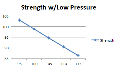
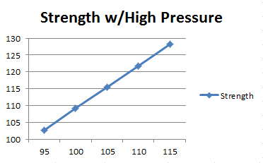
Dear Jim
Your blog is amazing! Makes everything more understandable for someone with no stats background! Thank you!
Hi Marlie, thanks so much for your nice comment. It means a lot to me because that’s my goal for the blog! I’m glad it’s been helpful for you.
First of all, thank you for the clear explanation. It is hard sometimes to find someone who can explain it in plain English!
Secondly, I still face an issue what to put on my axis in my research. I saw in your explanation that you put the dependent variable, the interaction term and one independent variable on the axis. My question is why you did not put both the independent variables that are in the interaction term, and the interaction term on the axis.
Already many thanks!
Hi Dan,
Thanks so much. I work really hard to find the simplest way to explain these concepts yet staying accurate!
Graphing relationships for multiple regression can get tricky. The problem is that the typical two-dimensional graph has only two-axes. So, you have to figure out the best way to arrange these two axes to produce a meaningful graph. This isn’t a problem for simple regression where you have one dependent variable and one independent variable. You can graph those two variables easily on fitted line plots. You have as many variables as you have axes.
Once you get to multiple regression you will have more than two variables (one DV, and at least 2 IVs, and possibly other terms such as interaction terms) than axes. You definitely want to include the dependent variable on an axis (typically the y-axis) because that is the variable you are creating the model for. Then, you can include one IV on the X-axis. At this point, you’ve used up your available axes! The solution is to use separate lines to represent another variable (as shown in the legend). That’s how you get the two IVs into the graph that you need for a two-way interaction. Then you just assess the patterns of those lines.
Instead, if I had put an IV on both X and Y-axes, the graph would not display the value of the DV. The whole point of regression/ANOVA is to explore the relationships with the DV. Consequently, the DV has to be on the graph.
I hope this helps clarify the graphs! The interaction plots I show in this post are the standard form for two-way interactions.
I see our replies crossed in cyberspace and are that we are similarly puzzled. I’m assuming you ran an ANOVA routine and that it gives you regression output automatically. Just out of curiosity, what if you were to convert your variables to 0/1 and ask your software to just run regression?
I used regression analysis in Minitab and it automatically creates the indicator variables behind the scenes. So, I just told it to fit the model. Depending on which level of each categorical variable that the software leaves out, you’d expect different numeric results (although, they’d tell the same story). You wouldn’t expect differences in what is and is not significant though. I wonder if STATA possibly uses sequential SS for one of it’s analyses? Minitab by default uses adjusted SS. Using Seq. SS could change which variables are significant. I was going to test that but haven’t tried yet.
However, I’m still puzzled as to why I got such different output when I transformed the data to 0/1 dummy variables, created an interaction variable, and then ran regression.
Mystery solved! It wasn’t an issue of the difference in software but rather in the type of model. I had asked Stata to run a regression model and got output that didn’t match up. However, when I ask Stata to run ANOVA (including the interaction term), I got output that matched yours. For other Stata users, the syntax to use is “anova enjoyment food condiment food#condiment”.
Hi Erick, thanks so much for the update! I had rerun the analysis to be sure that I hadn’t made a mistake, but it produced the same results in the blog post. I guess this goes this goes to show how crucial it is to know what your statistical software is doing exactly! I still wonder what produced the difference between the regression and the ANOVA model because they both use the same math underneath the hood? In other words, what is different between Stata’s regression and ANOVA model?
Dear Jim,
I found your blog while trying to find an answer to a reviewer comment to a paper I submitted.
So now I am looking for answers.
One of my hypothesis was on a moderated mediation model.
Considering the moderation I have (measured as continuous variables):
X=job demands
M (moderator)= team identification
Y= workplace bullying
The fact is that when I looked at the results the effect of X on Y is positive; the effect of M on Y is negative but my problem is that I have the interaction term (X*M) that is positive, while I (and especially the reviewer) was expecting a negative effect.
The graph makes sense to me (and partly the reviewer) but he/she is expecting that I am giving him/her some explanation about this positive interaction effect.
I hope you could help me in explaining me why and explain that to the reviewer!
Hi Michela,
I seem to have been encountering this question frequently as of late! The answer is that the coefficient for an interaction term really doesn’t mean much by itself. After all, the interaction term is a product of multiple variables in the model and the coefficient. Depending on the combination of variable values and the coefficient, a positive coefficient can actually represent a negative effect (i.e., if the product of the variable values is negative). Additionally, the overall combined effect of the main effect and interaction effect can be negative. It might be that the interaction effect just makes it a little less negative than it would’ve been otherwise. The interaction term is basically an adjustment to the main effects.
Also, realize that there is a bit of arbitrariness in the coefficient sign and value for the interaction effect when you use categorical variables. Linear models need to create indicator variables (0s and 1s) to represent the levels of the categorical variable. Then, the model leaves out the indicator variable for one level to avoid perfect multicollinearity. Suppose you have group A and group B. If the model includes the indicator variable for group A, then 1s represent group A and 0 represents not group A. Or, it could include the indicator variable for group B, then 1s represent group B and 0 represents not group B. If you have only two groups A and B, then the 1s and 0s are entirely flipped depending on which indicator variable the model includes. You can include either indicator variable and the overall results would be the same. However, the coefficient value will change including conceivably the sign! You can try changing which categorical level the software leaves out of the model, which doesn’t change the overall interpretation/significance of the results but can make the interpretation more intuitive.
Finally, it’s really hard to gain much meaning from an interaction coefficient itself for all the reasons above. However, you can see the effect of this term in the interaction plot. As long as the interaction plot makes sense theoretically, I wouldn’t worry much about the specific sign or value of the coefficient. I’d only be worried if the interaction plots didn’t make sense.
I hope this helps!
Jim, like many others here, I love your intuitive explanation.
I thought it would be a good exercise to replicate what you did in your example. (I’m using Stata, and I understand you don’t use that, but the results should still be the same.) Unfortunately, I’m having trouble replicating your results and I don’t know why. Using values of 0 and 1 for each of the IVs, I’m getting significant results for both of them and for the interaction variable, while you got NS results for one of the IVs.
I’ll paste the output below. (Sorry, the formatting got lost.)
. regress enjoyment food_01 condiment_01 food_cond
Source | SS df MS Number of obs = 80
————-+—————————— F( 3, 76) = 212.43
Model | 15974.9475 3 5324.98248 Prob > F = 0.0000
Residual | 1905.09733 76 25.0670701 R-squared = 0.8935
————-+—————————— Adj R-squared = 0.8892
Total | 17880.0448 79 226.329681 Root MSE = 5.0067
——————————————————————————
enjoyment | Coef. Std. Err. t P>|t| [95% Conf. Interval]
————-+—————————————————————-
food_01 | -28.29677 1.583258 -17.87 0.000 -31.45011 -25.14344
condiment_01 | -24.28908 1.583258 -15.34 0.000 -27.44241 -21.13574
food_cond | 56.02826 2.239065 25.02 0.000 51.56877 60.48774
_cons | 89.60569 1.119533 80.04 0.000 87.37594 91.83543
——————————————————————————
Any clue as to what’s I’m doing wrong?
Hi Erick, offhand I don’t know what could have happened. As you say, the results should be the same. I’ll take a closer look and see if I can figure anything out.
Thank you for the reply, Sir. I will do my best to interpret the interaction plot. 🙂
I do have 20 IV binary or categorical variables and one binary DV. My question is shall I check col linearity first and run bi variate analysis or otherwise. help me please
do have 20 IV binary or categorical variables and one binary DV. My question is shall I check col linearity first and run bi variate analysis or otherwise. help me please
Hi Sir. Thank you for this wonderful post as this is very helpful. But I still can’t seem to understand or interpret my interaction plot. My main effects are significant and my interaction effect are also significant but then looking at the regression coefficient (result from SPSS), moderator(IV2) is a negative significant predictor of DV but looking at my interaction plot, they are both positive significant predictor? I’m not sure if you get it because I am also having difficulty explaining the situation because I am just a beginner when it comes to psychological statistics. Thank you in advance, Sir!
Hi Mei, I don’t understand your scenario completely. However, there is nothing wrong with having positive coefficients for main effects and negative coefficients for interaction effects. When you have significant interaction effects, then the total effect is the main effect plus interaction effect. In some cases, the interaction effect adds to the main effect but sometimes it subtracts from it. It’s ok either way. I find that assessing the interaction plots is the easiest way to interpret the results when you have significant interaction effects.
Thank you for the long post Jim!
I used a cog regression model and the results is hazard ratio’s. The trial is physical activity vs control. And we are doing a subgroup analysis with the supplement.
The above table shows for Users the CI is 1.40 ( .85 to 2.3) and not significant.
For nonusers, the HR shows 0.61 ( 0.46-.80) and significant.
And the interaction between these two is significant. My question is isn’t this an example of qualitative interaction where the direction is opposite for users vs non-users. Like if you plot the forest plot, the lines are on 2 sides of no difference line.?
Hi Anoop,
The interesting thing about statistics is that the analyses are use in a wide array of fields. Often, these fields develop their own terminology for things. In this case, I wasn’t familiar with the term qualitative interaction, but it seems to be used in medical research. I’ve read that a qualitative interaction occurs when one treatment is better for some subsets of patients while another treatment is better for another subset of patients. It sounds like a qualitative interaction occurs when there is a change in direction of treatment effects. A non-crossover interaction applies to situations where there is a change in magnitude among subsets but not of direction.
So, I learned something new about how different fields apply different terminology to statistical concepts!
I’m not sure why you’d have only two hazard ratios when you know that the interaction effect is significant? Right there you know that you can’t interpret the main effect for supplement usage without knowing the physical activity level. It seems like you’d need 4 hazard ratios.
As for whether this classifies as a qualitative interaction given the definition above, you’ll first have to determine whether those differences between the three groups I identified before are both statistically significant and practically significant. If the answers to both questions are yes, then it would seem to be a qualatative interaction. However, if either answer is no, then I don’t think it would. And, I’m going by your dependent variable. If you want to answer that using hazard ratios, you’d need four of them as I indicate above. You can’t answer that question with only two ratios.
I hope this helps!
Hey Jim,
Not sure why ur posting doesn’t show. But it shows in my email.
This is a trial is looking at if physical activity vs Control can reduce physical disability. We are looking at a certain supplement users vs nonusers in the trial. Interaction was significant ( p=.003)
PA C
Users 7.1 6.1 HR 1.40 (.85 – 2.3)
Nonusers 5.4 10.2 HR 0.61(.46 – 0.80)
How do you interpret this result?
Thank you so much. Also you should start a youtube page. We need more people like you in this world 🙂
Hi again Anoop,
I checked and I see my comment showing up under yours. I think it might be a browser caching thing that is causing you not to see my reply on the blog post. Refresh might do the trick.
At any rate, this example will also show the importance of several other concerns in statistics–namely understanding the subject area, the variables involved, and statistical vs. practical significance. So, with that said, let’s take a look at your results!
I’m not sure what the dependent variable is, but I’ll assume that higher values represent a greater degree of disability. If that’s not the case, you got really strange results! In the interaction table you provided, I see three group means that are roughly equal and one that stands out. I’m not sure if the differences between any of those three group means (5.4, 6.1, and 7.1) are statistically significant. You can perform a post hoc analysis in ANOVA to check this (I plan to write a blog post about that at some point). Even if they are significant, you have to ask yourself if those differences are practically significant given your knowledge of the subject area and the dependent variable. I don’t know the answer to that.
And, then there is the one group mean (10.2) that is noticeably different than the other three groups. To me, it looks like that subjects in the control group who don’t use the supplement have particularly bad results. And, the other three groups might represent a better outcome. Again, use your subject-area knowledge to determine how meaningful this result is in a practical sense.
If that’s the case, it suggests to me that subjects have better outcomes as long as they use the supplement and/or engage in physical activity. In other words, the worst case is to not do either the activity or use the supplement. If you do one or both of physical activity and supplement usage, you seem to be better off in an approximately equal manner. And, again, I don’t know if the differences between the other three outcomes are statistically significant and practically significant. In other words, those differences could just represent random sample error and/or not be meaningful in a practical sense.
I hope this clarifies things! And, yes, I do plan to start a YouTube channel at some point. I need to finish a book that I’m working on first though!
Take care,
Jim
Hi Jim,
I have an interaction significant ( 0.004) for supplement use and physical activity interaction. The nonusers had a Hazard Ratio 0f 0.61(.46-0.80) ( lower risk) where users had a HR 1.40 (.85-2.3) ( high risk). My question is although it looks like a qualitative interaction ( opposite in direction), since the users CI crosses margin of no difference, how do you interpret it? Can we say users had a higher hazard when combined with PA?
Thank you
HI Anoop,
I can’t interpret the main effect of supplement use without understanding the interaction effect. Can you share, the hazard ratios for your interaction. In other words, the ratios for the following groups: user/high activity, user/low activity, non-user/high activity, and non-user low-activity.
I don’t know how you recorded activity, so those groups are just an example. Then we can see how to interpret it!
Thanks!
Jim
Hi Jim,
Thanks for your reply. Yes that was one of the problems that was pointed out in my dissertation; was that it did not have a control group that was compared to :/ It was due to the fact that alongside time constraints, the sample size was already so small so it was difficult to get enough people to make 3 separate groups :/ So should am i wrong to accept the hypothesis that both RT and MD has a positive effect on wellbeing levels? Or do i have to reject that as i did not have a control group?
Kind Regards,
Michela
Hi Michela,
Unfortunately, it is hard to draw any conclusions about the treatments. It’s possible that both had the same positive effect on well being. However, it’s also possible that neither had an effect and instead it was entirely the passage of time. I definitely understand how it is hard to work with a small sample size!
If other researchers have studied the same treatments, you can evaluate their results. That might lend support towards your notion. But, that’s a tenuous connection without a control group.
Best wishes to you!
Jim
Hi Jim,
This blog post is so useful thank you very much! I have however still fail to interpret one of my statistics output. I carried out a two-way mixed ANOVA analysis and inputted these data:
– between-subject variable is two therapy techniques (MD and RT)
– within-subject variable (Time with 3 levels: pre, mid and post)
– dependant variable was well-being scores.
I ran the analysis and found that for the between-subject variables there were no significant difference between the well-being scores for MD and RT therapies. However when looking at my within-subject variables. The table stated that there was a significant main effect of Time on wellbeing scores but no significant interaction between Time*Therapy on well-being scores.
Am i right in implying that with the significant main effect of time it basically states that over-time, wellbeing scores improved, independent of the therapy techniques. Can i then conclude RT and MD positively improved well-being in general and that not one is better then the other? Or is that wrong? As one of my hypothesis states that MD and RT will have a positive effect on wellbeing scores.
Thank you so much for taking time to read this and helping me !!
Michela
Hi Michela,
Your interpretation sounds correct. The data you have suggests that as time passes, well being increases. You don’t have evidence that either treatment works better than the other. Often you’d include a control group (no treatment). It’s possible that there is only a time effect and no treatment effect. A control group would help you establish whether it was the passage of time and/or the treatments.
In other words, right now it could be that both treatments are equally effective. But, it’s also possible that neither treatment is effective and it’s only the passage of time–as the saying goes, time heals all wounds!
Hi Jim!
Thank you very much for your blog site, you explain things well and understandable, thank you for that!!
I would still like to make sure, that I understand correctly what you said before.. I am running a repeated measures ANOVA and I am struggling with interpretations of interactions. So, is it so, that if the interaction effect is not significant, then you should not interpret the multivariate comparisons between groups? I have a model with 5 groups and I am trying to see if there are any differences between them in the change of X variable in two time points. In multivariate tests it shows that the change would be different in one of the groups (also the plot figure shows that), but the overall interaction effect is significant. So what would be the right way to interpret the results? Just say that there were no significant interaction i.e. tha change was similar in all groups, or say that one group was different but the interaction effetc was not (for some reason?).
Thank you already for your answer!
Satu
Hello jim,
What if want to know 1. How does Icecream and hotdog affect enjoyment by itself
2. How does icecream and hotdog affect enjoyment when condiments are included?
In this case, isn’t both the main effect and interaction are equally important for a researcher?
Hi Anoop,
Great questions! You can see how ice cream and hot dog affect enjoyment by themselves by looking at the main effects plot. This plot shows the enjoyment level that each food produces is approximately equal.
Yes, understanding main effects like these are important. However, when there are significant interaction effects, you know that the main effects don’t tell the full story. In this case, the main effect for, say hot dog, doesn’t describe the full effect on enjoyment. The interaction term includes hot dog, so you know that some of hot dog’s effect is also in the interaction. If you ignore that, you risk misinterpreting the results. As I point out in the blog, if you go only by main effects, you’ll choose a hot dog . . . with chocolate sauce. You’d pick the chocolate sauce because it’s main effect is larger than mustard’s main effect.
To see how ice cream and hot dogs affect enjoyment when you include the interaction effect, just look at the interaction plot. The four points on that plot show the mean enjoyment for all four possible combinations of hot dog/ice cream with chocolate sauce/mustard. It displays the total effects of main effects plus interaction effects. For example, the interaction plot shows that for hot dogs with mustard, the mean enjoyment is about 90 units (the top-left red dot in the graph). Alternatively, you could enter values into the equation to obtain the same values.
I’d agree that understanding both main effects and interaction effects are important. My point is that when you have significant interaction effects, don’t look at only the main effects because that can lead you astray!
how does interaction affect my study statistically
Hi Demmie, this is the correct post for finding that answer. Read through it and you’ll find the answer you’re looking for. If you have a more specific question, please don’t hesitate to ask!
Thanks for your help and your quick response. I really appreciate.
Again, THANK YOU.
Sincere,
Ting-Chun
Hi Jim,
May I ask what reference about interaction effect do you suggest to study?
I want to know more about interaction effect in clinical trial.
Thank you.
Sincere,
Ting-Chun
Hi Ting-Chun, most any textbook about regression analysis, ANOVA, or linear models in general will explain interaction effects. My preferred source is Applied Linear Regression Models. That’s a huge textbook of 1400 pages, but that’s why I like it! I don’t have a reference specifically for interaction effects, but would recommend something that discusses linear models in all of its aspects.
I hope this helps!
Jim
Thanks Jim for your quick response and comprehensive explanation..
Thank Jim, your explanation is very nice to follow, by the way, i have a model e.e. growth=average year of schooling +political stability+average year of schooling*political stability. the stata output gives individual coefficient positive while interactive coefficient negative. unfortunately i been asked by the reviewer to explain why interaction sign is negative any statistical or theoretical explanation please.
Hi Hakim, it’s difficult to interpret the coefficients for interaction terms directly. However, I can tell you that there is nothing at all odd about having a negative sign for an interaction term. Interaction terms modify the main effects. Sometimes it adds to them while other times it subtracts. It all depends on the nature of what you’re studying.
I’d suggest creating interaction plots, like I do in this post, because they’re much easier to understand than the interaction coefficients. Look through the plots to see whether they make sense given your understanding of the subject-area. These plots are a graphical representation of the interaction terms. Therefore, if the plots make sense, your model is good to go. If they don’t, then you need to figure out what happened. I think the reviewers will find the plots easier to understand than the coefficient.
I hope this helps!
Thanks for your help. I really appreciate.
Might need your help again after I finished the post hoc.
Hope you okay with that. Haha.
Again, THANK YOU.
Sincere,
Bill
Hello. Jim. Thank for your great article.
Sorry in advance for my English. Moreover, my understanding for SPSS and stat is quite limited so some question might be silly.
I’m doing 4×5 factorial ANOVA. One of the test has Sig. interaction effect but I don’t know what exact method should I interpret it. Some told that I need to do simple main effect test, some told that Post Hoc is enough so I’m quite confused.
Another test the graph shown some cross-over line (because there are a lot of levels of iv) but the sig. value is 0.069 = not significant interaction effect right?. However I’ve read that if the line crossed, the interaction is exist. So how should I summarize?
I’m willing to send the information for you if u need.
Thank you.
Bill
Hi Bill,
You have some excellent questions!
When you have a significant interaction effect, you know you can’t interpret the main effects without considering the interaction effects. As I show in the post, interaction effects are an “it depends” effect. The interpretation for one factor depends on the value of another factor. If you don’t assess the interaction effect, you might end up putting ketchup on your ice cream!
Assessing the Post Hoc test results can be fine by itself as long as you include the interaction term in the ad hoc test. Taking that approach, you’ll see the groupings based on the interaction term and know which groups are significantly different from each other. I also like to graph the interaction plots (as I do in this post) because it provides a great graphical overview of the interaction effect.
There’s an important point about graphs. They can be very valuable in helping you understand your results. However, they are not a statistical test for your data. An interaction plot can show non-parallel lines even when the interaction effect is not significant. When you work with sample data, there’s always the chance that sample error can produce patterns in your sample that don’t exist in the population. Statistical tests help you distinguish between real effects and sample error. These tests indicate when you have sufficient evidence to conclude that an effect exists in the population.
When you have crossed lines in an interaction plot but the test results are not statistically significant, it tells you that you don’t have enough evidence to conclude that the interaction effect actually exists in the population. Basically, the graph says that the effect exists in the sample data but the statistical test says that you don’t have enough evidence to conclude that it also exists in the population. If you were to collect another random sample from the same population, it would not be surprising if that pattern went away!
I hope this helps!
This is one of the best explanations I have read to explain ‘interactions’. Thanks!
Thanks so much, Saheeda! Your kind words mean a lot to me! I’m glad it was helpful.
Hi Jim,
Thankyou for such a quick and helpful response!
Graphing the interaction effect is actually what confused me when it came to interpretting my results. The conditions are actually parallel to one another, there is no cross over. The gradient for the comedy condition is almost zero, whereas, there is a dramatic drop in rating of boredom between time 1 and time 2 for the nature video.
With this in mind does the interpretation then mean: A difference in boredom is found across time depending on condition. Therefore, only if you are watching the nature video will you become significantly more bored at time 2. Will I need to conduct a t-test to conform this?
Many thanks!
Courtney
Hi Courtney,
You bet! 🙂
Technically, a significant interaction effect means that the difference in slopes is statistically significant. The lines don’t actually have to cross on your graph–just have different slopes. Well, having different slopes means that the lines must cross at some point theoretically even if that point isn’t displayed on your graph.
As for the interpretation, the zero slope for comedy indicates that as time passes, there is no tendency to become more or less bored. However, for nature videos, as time passes, there is a tendency to become more bored. (I’m assuming that the drop in rating that you mention corresponds to “becomes more bored”.) This difference in tendencies is statistically significant. The significant interaction indicates that the relationship between the passage of time and boredom depends on the type of video the subjects watch.
Again, an interaction effect is an “it depends” effect. Do the subjects become more bored over time? It depends on what type of video they watch! You can’t answer that question without knowing which video they watch.
So, the interaction tells you that the difference in slopes is statistically significant, which is different than the whether the difference between group means are statistically significant. To identify the specific differences between group means that are statistically significant, you’ll need to perform a post hoc test–such as Tukey’s test. These tests control the joint error rate because as you increase the number of group comparisons, the chance of a Type I error (false positive) increases if you don’t control it. I don’t have a blog post on this topic yet but plan to write one.
The interaction term tells you that the relationship changes while the post hoc test tells you whether the difference between specific group means is statistically significant.
Hi Jim,
Thankyou so much for your quick and helpful response, it really means a lot!
This is what initially confused me when it came to interpreting my results, looking at my interaction graph there was no cross over. Both conditions are more or less parallel with one another, the gradient between time 1 and time 2 for comedy is almost 0. However, there is quite the drop for the nature video in the boredom rating at time 2.
Because the interaction graph does not cross over, does this mean that only in the Nature video does the boredom decrease significantly at Time 2? Will I need to conduct a t-test to check this?
Many thanks!
Courtney
Hi Jim,
Thankyou for this post, I found it incredibly helpful.
I am having trouble interpreting my own results of a two-way repeated ANOVA and was wondering if you could help me out.
Participants were exposed to two different videos, controlled with a counter balance. Video 1 consisted of a comedy sketch, while video 2 was of a nature documentary. Every 2 mins the participants had to indicate on a likert scale how Bored they felt at the time. For the analysis I averaged the boredom score over the first and second half of the video.
IV1: Video (Comedy vs Nature)
IV2: Time (Time 1 vs Time 2)
DV: Boredom score
My analysis output reveals a significant main effect of video p<.000, and non significant effect for time p=.192. However I have an effect of interaction for video*time, p<.000.
How would you go about interpreting these results?
Thanks in advance!
Hi Courtney,
I’m happy to hear that you found this post helpful!
The first thing that I’d recommend is graphing your results using an interactions plot like I do in this post. That’s the easiest way to understand interactions. It’s great that you’ve done the ANOVA test because you already know that whatever pattern you see in the plot is, in fact, statistically significant. Given the significance, I can conclude the lines on your plot won’t be parallel.
For your results, you can state them one of two ways. Both ways are equally valid from a statistical standpoint. However, one way might make more sense than the other given your study area or what you’re trying to emphasize.
1) The relationship between Video and Boredom depends on Time. Or:
2) The relationship between Time and Boredome depends on Video.
For the sake of illustration, let’s go with #2. You might be able to draw the conclusion along the lines of: As subjects progress from time 1 to time 2, the average boredom score increases more slowly for those who watch comedy compared to those who watch a nature documentary. Of course, you’d have to adapt the wording to match your actual results. That’s the type of conclusion that you can draw, and you’re able to say that it is statistically significant given the p-value for the interaction term.
Given that the interaction term is significant, you don’t need to interpret the main effects terms at all. And, it’s no problem that one of the main effects is not significant.
I hope this helps!
Hello Jim!
Thanks for making such very clear posts. I tutor students with stats and its really tough to find good easy to follow material that EVERYONE can get. So to stumble on such a clear explanation is a breath of fresh air 😀
Now I recently saw in one of my students powerpoints that they are taught they have to redo the ANOVA analysis without the interaction if the interaction is not significant. Maybe i’ve always missed something but I have never heard of this before. Does this sound familiar to you and if so can you explain to me why this is?
thanks!
Susanne
Hi Susanne, thanks so much for your kind words. They mean a lot to me–especially coming from a stats tutor!
I have always heard that you should not include the interaction term when it is not significant. The reason being is that when you include insignificant terms in your model, it can reduce the precision of the estimates. Generally, you want to leave as many degrees of freedom for the error as you can.
Hi Jim,
Thanks for your explanation! It was really useful. I have a couple of follow-up questions. Let’s suppose a situation with 2 regression models, both of which have the exact same variables, except the second model has an additional interaction term between two variables already in the first model.
1. Now comparing the 2 regression equations, why do coefficients of other variables (apart from the interaction term and the 2 variables used to create the interaction term) change?
2. How do we compare and interpret the change in coefficients of variables which were used to create the interaction term in the first and second models?
Let me know in case it’s better for me to explain with an example here.
Thanks!
Hi Shruti,
I think I understand your questions.
1) Any time you add new terms in the model, the coefficients can change. Some of this occurs because the new term accounts for some of the variance that was previously accounted for by the other terms, which causes their coefficients to change. So, some change is normal. The changes can tend to be larger and more erratic when the model terms are correlated. The interaction term is clearly correlated with the variables that are included in the interaction. When you include an interaction term, you can help avoid this by standardizing your continuous variables.
2) I have heard about cases where analysts try to interpret the changes in coefficients when you add new terms. My take on this is that the changes are not very informative. Let’s assume that your interaction term is a valuable addition to the model. In that case, you can conclude the model without the interaction term is not as good of a model and it’s coefficient estimates might well be biased. Consequently, I wouldn’t attribute much meaning to the change in coefficient values other than your new model with the interaction term is likely to better.
However, one caveat, I believe there are fields that do place value in understanding those changes. I’m not sure that I agree, but if your field is one that has this practice, you should probably check with an expert.
I hope I covered everything!
Hi, Jim!
Thank you again for your willingness! Unfortunately, I can’t /don’t know how to post the plot in the comments… If you are willing, you can contact me by email so I can send it to you, plus the results of the regression or whatever information that could be helpful.
Thank you!
Hi Jim,
first of all… thank you very much for your early response!
And after that… I am so sorry! I forgot to explain that I work with lizards, not with humans. My measurement of body length (logLCC) corresponds to the log-transformed Snout-Vent Length (logSVL, whose acronym in spanish, given that it’s my mothertongue, is LCC; I forgot to translate it!). The relationship among these two variables tend to be linear.
So, in these animals, the regression of logSVL and logweight is a common and standardized method to assess body condition. Residuals from this regression are used to assess body condition; if they’re positive the animal is more “chubby” (better condition) and, if they’re negative, the animal is more “skinny” (worse condition). The aim of my ANCOVA is to compare the effect of age on this regression.
Anyway, following your advice I created an interaction plot which displays two lines, one for each level of the age factor. The two lines cross in a certain middle point, diverging prior and after that point. Thanks to your detailed answer, I understand that this means that age interacts somehow with body length (what sounds logical, as lizards grow together with aging), but I still don’t know how to interpret this in relation to body condition (regression).
Thanks again for your detailed, kind and early response!
You’re very welcome! And, subject area knowledge and standards definitely should guide your model building. I always enjoy learning how others use these types of analysis. And, that’s interesting actually using the residuals to assess a specimen’s health!
If you can, and are willing, post the interaction plot, I can take a stab at interpreting it. (I know I can post images in these comments but I’m not sure about other users.) Basically, the relationship between body length and weight depends on the age factor. Or, stated another way, you can’t use body length to predict weight until you know the age.
Hi, Jim!
I have a sort of somehow interaction-related question, but I didn’t know where to post it, so this entry seemed the most adequate to me.
I work with R and I would like to use an ANCOVA to evaluate the effect of a factor (age, for example, with two levels, adult and subadult) in the regression of body length (log transformed, logLCC) and weight (log transformed, logweight). This regression measures body condition of an individual (higher weights at same lenghts indicate a better condition, that is, sort of “fluffyness”).
So, when I run the analysis:
aov(logweight~logLCC*age)
I obtain a significant interaction between logLCC:age (p=0.0068). I understand this means that slopes for each age class are not paralell. However, the factor age alone it’s not significant (p=0.2059).
What does this mean? How is it interpreted?
I have tried deleting the interaction from the model, but it loses a lot of explicative power (p=0.0068). So, what should I do? I am quite lost with this issue…
Thank you so much in advance,
Alicia
Hi Alicia!
First, before I get into the interaction effect, a comment about the model in general. I don’t know if you’re analyzing human weight or not. But, I’ve modeled Percent Body Fat and BMI. While I was doing that, I had to decide whether to use Height, Weight, and Height*Weight as the independent variables and interaction effect or should I use body mass index (BMI). I found that both models fit equally as well but I went ahead with BMI because I could graph it. I did have to include a polynomial term because the relationship was curvilinear. I notice that you’re using a log transformation. That might well be just fine and necessary. But, I found that I didn’t need to go that route. Just some food for thought. You can read about this BMI and %body fat model.
Ok, so on to your interaction effect. It’s not problematic at all that the main effect for age is not significant. In fact, when you have a significant interaction you shouldn’t try to interpret the main effect alone anyway. Now, if it had been significant and you wanted determine the entire effect of age, you would’ve had to assess both the main effect and the interaction effect together. Now, you just need assess the interaction effect alone. But, it’s always easiest to interpret interaction effects with graphs, as I do in this blog post.
In the post, I show examples of interaction plots with two factors and another with two continuous variables. However, you can certainly create an interaction plot for a factor * continuous variable. For your model, this type of graph will display two lines–one for each level of the age factor. Because you already know the interaction term is significant, the difference between the two slopes is statistically significant. (If the main effect had been significant, the interaction plot would have included it in the calculations as well–but it is fine that it’s not significant.)
It sounds like you should leave the interaction effect in the model. Some analysts will also include the main effects in the model when they are included in a significant interaction effect even if the main effect is not significant by itself (e.g., age). I could go either way on that issue myself. Just be sure that the interaction makes theoretical/common sense for your study area. But, I don’t see any reason for concern. The insignificant main effect is not a problem.
I hope this helps!
Hi Jim,
Thank for the valuable tutorial.
I have 2 questions as follows:
1. In more complex study areas, the independent variables might interact with each other. What do you mean by complex area? Is it social science?
2. I have run Mancova and observed that results of two-way = interaction. I found that SPSS does not run post-hoc. Can I use the t-test after that?
My model is factorial design (2 levels of X1, 2 levels of X2, and 2 levels of X3) on Y.
I report in paper for two-way and three way interaction on below. Is it ok?
Two-way interaction
Among the X2 level 1 group, the mean of Y among subjects who viewed X3 level 2 (adjusted M = xxx, SE =xxx) is significantly higher than those who viewed X3 level 1 (adjusted M = xxx, SE = xxx) with t(xx) = xx, p < xx.
three-way interaction
Among the subjects who viewed the X3 level 2, the mean of Y of the subjects who expressed X1 level 2 (adjusted M = xxx, SE = xxx) is significantly greater than those who expressed X1 level 1 (adjusted M = xxx, SE = xxx) for those who had X2 level 1 [t(xx) = xxx, p < xxx].
Thank you in advance
Hi Tanikan,
Thanks for the great questions!
Regarding more and less complex study areas, in the context of this post, I’m simply referring to subject matter where only main effects are statistically significant as being simpler. And, subject areas where interaction effects are significant as more complex. I’m calling them more complex because the relationship between X and Y is not constant. Instead, that relationship depends on at least one other variable. It’s just not as simple.
I would not use t-tests for that purpose. I’m surprised if SPSS can’t perform post-hoc tests when there are interaction effects–but I use other statistical software more frequently. With your factorial design, there will be multiple groups based on the interactions of your factors. As you compare more groups, the need for controlling the family/joint/simultaneous error rate becomes even more important. Without controlling for that joint error rate, the probability that at least one of the many comparisons will be a false positive increases. T-tests don’t control that joint error rate. It’s important to use a post hoc test.
At least for the two-way interaction effects, I highly recommend using an interaction plot (as shown in this post) to accompany your findings. I find that those graphs are particularly helpful in clarifying the results. Of course, that graph doesn’t tell you which specific differences between groups are statistically significant. The post hoc tests for those groups will identify the significant differences.
I hope this helps!
Great work Jim! People get very vague idea whenever they look at google to learn the basic about interaction in statistics. Your writing is a must see and excellent work that demonstrated the basic of interaction. Thanks heaps.
Hi Yeasin, thank you! That means a lot to me!
Thanks for help, I appreciate it!
Your explanation is really great! Thank you so much. I totally will recommend you to my friends
You’re very welcome! Thank you for recommending me to your friends!
Hello,
I am interested how to read for interaction effect if we just have a table of observations, for example
A B C
2 4 7
4 7 8
6 9 13
In the lecture I attended this was explained as “differences between differences” but I didn’t get what this refers to.
Thanks
Hi Luka, it’s impossible to for me to interpret those observations because I don’t know the relationships between the variables and there are far too few observations.
In general, you can think of an interaction effect as an “it depends” effect as I describe in this blog post. Suppose you have two independent variables X1 and X2 and the dependent variable Y. If the relationship between X1 and Y changes based on the value of X2, that’s an interaction effect. The size of the X1 effect depends on the value of X2. Read through the post to see how this works in action. The value of the interaction term for each observation is the product of X1 and X2 (X1*X2).
An effect is the difference in the mean value of Y for different values of X. So, if the interaction effect is significant, you know that the differences of Y based on X will vary based on some other variable. I think that’s what your instructor meant by the differences between differences. I tend to think of it more as the relationship between X1 and Y depends on the value of X2. If you plot a fitted line for X1 and Y, you can think of it as the slope of the line changes based on X2. There’s a link in this blog post to another blog post that shows how that works.
I hope this helps!
Hi Jim, thank you very much for your post. My question is how do you interpret an insignificant interaction of a categorical and a continuous variable, when the main effects for both variables are significant? For the sake of simplicity if our logit equation is as follows Friendliness = α + βAge + βDog + βAge*Dog. Where Friendliness and Dog are coded as dummy variables that take the values of either 1 or 0 depending on the case. So if all but the interaction term, βAge*Dog, is significant, does that mean the probability of a dog being friendly is independent of its age?
If the Age variable is significant, then you know that friendliness is associated with age, and dog is as well if that variable is significant. A significant interaction effect indicates that the effect of one variable on the dependent variable depends on the value of another variable. In your example, lets assume that the interaction effect was significant. This tells you that the relationship between age and friendliness changes based on the value of the dog variable. In that case, it’s not a fixed relationship or effect size. (It’s also valid to say that the relationship between dog and friendliness changes based on the value of age.)
Now, in your case, the interaction effect is not significant but the two main effects are significant. This tells you that there is a relationship between age and friendliness and a relationship between dog and friendliness. However, the exact nature of those relationships DO NOT change based on the value of the other variable. Those two variables affect the probability of observing the event in the outcome variable, but one independent variable doesn’t affect the relationship between the other independent variable and the dependent variable.
The fact that you have one categorical variable and a continuous variable makes it easier to picture. Picture a different regression line for each level of the categorical variable. These fitted lines display the relationship between the continuous independent variable and the response for each level of dog. A significant interaction effect indicates that the differences between those slopes are statistically significant. An insignificant interaction effect indicates that there is insufficient evidence to conclude that the slopes are different. I actually show an example of this situation (though not with a logistic model) that should help.
I hope that makes it more clear!
what is the command for conintuous by continuous variables interaction plot in stata?
Thanks
Hi, I’ve never used Stata myself, but I’ve seen people use “twoway contour” to plot two-way interaction effects in Stata. Might be a good place to start!
what does it mean when I have a significant interaction effect only when i omit the main effects of the independent variables (by choosing the interaction effect in “MODEL” in SPSS). it is “legal” to report the interaction effect without reporting the main effects?
Hi Mona,
That is a bit tricky.
If you had one model where the main effects are not significant, but the interaction effects are significant, that is perfectly fine.
However, it sounds like in your case you have to decide between the main effects or the interaction effects. Models where the statistical significance of terms change based on the specific terms in the model are always difficult cases. This problem often occurs (but is not limited to) in cases where you multicollinearity–so you might check on that.
This type of decision always comes down to subject area knowledge. Use your expertise, theory, other studies, etc to determine what course of action is correct. It might be OK to do what you suggest. On the other, perhaps including the main effects is the correct route.
Jim
Thank you for amazing posts. the way you express concepts is matchless.
You’re very welcome! I’m glad they’re helpful!
Can I know which software did you use, because I use SPSS, but the result was not the same with you.
Hi, I’m using Minitab statistical software. I’m not sure why the results would be different. A couple of possibilities come to mind. Minitab presents the fitted means rather than raw data means–I’m not sure which values SPSS present. Minitab doesn’t fit the model using standardized variables, which SPSS might. I don’t have SPSS myself, otherwise I’d try it out. I do have confidence that Minitab is calculating the correct values. There must be some methodology difference.