Exponential Distribution: Uses, Parameters & Examples

What is the Exponential Distribution?

The exponential distribution is a right-skewed continuous probability distribution that models variables in which small values occur more frequently than higher values. It is a unimodal distribution where small values have relatively high probabilities, which consistently decline as data values increase. Statisticians use the exponential distribution to model the amount of change in people’s pockets, the length of phone calls, and sales totals for customers. In all these cases, small values are more likely than larger values.

Analysts frequently use the exponential distribution to model the amount of time between independent events. In this type of study, the probability density function assumes that events occur at a constant rate on average over time. For example, reliability analysts use this distribution to model failure times.

Related posts: Understanding Probability Distributions and Skewed Distributions

The Memoryless Nature of the Exponential Distribution

The exponential distribution is a “memoryless” distribution. Memoryless is a distribution characteristic that indicates the time for the next event does not depend on how much time has elapsed. For a memoryless process, the probability of an event happening one minute from now does not depend on when you start watching for the event. Alternatively, the likelihood of when the event occurs next does not depend on when it happened previously.

For example, after observing a bank teller work with a customer for a minute, the probability that the transaction concludes in the next minute is the same as a minute ago.

The exponential distribution has this memoryless property because the probability of an event occurring within a specified timeframe is not conditional on how long you’ve already been waiting for the event to occur. It describes the time between events in a Poisson process. This type of process has independent events that occur at a constant average rate.

In the shape parameter section, you’ll learn more about how the exponential and Poisson distributions are related.

For discrete data, the geometric distribution is similar to the exponential distribution because it is also memoryless.

Related posts: Poisson Distribution and Geometric Distribution

When to Use the Exponential Distribution

The exponential distribution assumes that small values occur more frequently than large values. Consequently, it can model things like wait times, transaction times, and failure times. It can also model other variables, such as the size of orders at convenience stores.

Consider whether the memoryless characteristic of events occurring independently at a constant average rate applies to your subject area.

Memorylessness is not valid for all subject areas, preventing the exponential distribution from modeling some phenomena. For instance, machines tend to wear out over time, causing failure rates to increase as time passes. However, accidents generally occur independently at a fixed rate.  When an accident doesn’t happen during one day, it doesn’t indicate that an accident is more or less likely to happen the next day.

This distribution assumes that the average time between events remains constant. Consequently, you cannot use the exponential distribution when the expected time for events increases or decreases as time passes. Other distributions, such as the Weibull distribution, are appropriate in those cases. Using the exponential distribution in reliability studies requires the process to have a consistent failure rate over time.

To determine which probability distribution best fits your data, read my post Identifying the Distribution of Your Data.

Exponential Distribution Parameters

There are two versions of the exponential distribution. The two-parameter variety, predictably, has two parameters, scale and threshold. When analysts set the threshold parameter to zero, it becomes a one-parameter exponential distribution. Let’s see how these parameters work!

Threshold Parameter

The threshold parameter defines the lowest possible value in an exponential distribution. Some analysts refer to this parameter as the location. All values must be greater than the threshold. Consequently, negative threshold values let the distribution to handle both negative and positive values. Zero allows the distribution to contain only positive values. A one-parameter exponential distribution simply has the threshold set to zero. Statisticians denote the threshold parameter using θ.

Suppose you measure transaction times in minutes, and the exponential distribution has a threshold value of 3. This condition indicates that transaction times cannot be less than three minutes.

When you hold the scale parameter constant, the threshold shifts the distribution left and right, as shown below.

Scale Parameter (β)

The scale parameter determines how quickly the probabilities for higher values or longer times (depending on what you’re modeling) decreases. The value of the scale parameter is the mean of the distribution, making it the expected value. In the most common use case for the exponential distribution, this parameter represents the mean time until the event occurs. Statisticians denote this parameter using beta (β).

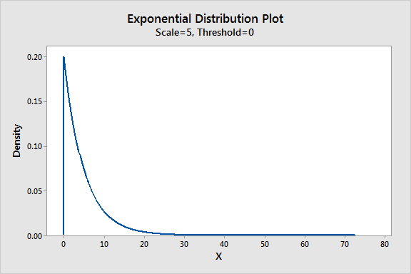
For example, if you measure the amount of time bank clerks spend with a customer in minutes and the scale parameter equals 5, it indicates that they spend an average of five minutes with each customer.

Decay or Hazard Rate Parameter (λ)

Alternatively, analysts can use the decay rate/hazard rate form of the parameter, lambda (λ), for the exponential distribution. Lambda is also the mean rate of occurrence during one unit of time in the Poisson distribution. To convert between the scale (β) and decay rate (λ) forms of the parameter, use the following equations:

• β = 1 / λ
• λ = 1 / β

They are reciprocals. Let’s return to our example of the clerks who spend an average of five minutes with each customer (β = 5) to understand why. An equivalent way to state it is that clerks finish one-fifth of a customer’s transaction in one minute on average (λ = 1 / 5 = 0.20).

The graph below displays this distribution. Note that the decay rate parameter will always be the maximum value on the y-axis, which is 0.20 in this example (β = 5, λ = 0.20).

The scale parameter represents the variability present in the distribution. Changing the scale parameter affects how far the probability distribution stretches out. As you increase the scale, the distribution stretches further right, and the height decreases. Decreasing the scale shrinks the distribution to the left and increases its peak, as shown below.

Related post: Measures of Variability

Comparing the Exponential, Poisson, and Gamma Distributions

As you’ve seen throughout this post, the exponential and Poisson distributions are related. In fact, these two distributions and the gamma distribution are related because they all model different characteristics of a Poisson process. These three probability distributions can all use lambda as a parameter that represents the constant average rate of occurrence for independent events. Here’s how these distributions compare.

The exponential distribution models the time between events. Time is a continuous variable and the exponential distribution is, correspondingly, a continuous probability distribution.

While the exponential distribution models the time until the next event occurs, the related gamma distribution models the time until the k^th event occurs, where k is the shape parameter.

Conversely, the Poisson distribution models the count of events within a fixed amount of time. A count is a discrete variable and the Poisson distribution is a discrete probability distribution.