What is the Gamma Distribution?
The gamma distribution is a continuous probability distribution that models right-skewed data. Statisticians have used this distribution to model cancer rates, insurance claims, and rainfall. Additionally, the gamma distribution is similar to the exponential distribution, and you can use it to model the same types of phenomena: failure times, wait times, service times, etc.
 The most frequent use case for the gamma distribution is to model the time between independent events that occur at a constant average rate. Using this distribution, analysts can specify the number of events, such as modeling the time until the 2nd or 3rd accident occurs. In this context, reliability analysts use the gamma distribution to model failure times.
The gamma distribution is a generalization of the exponential distribution. The gamma distribution can model the elapsed time between various numbers of events. Conversely, the exponential distribution can model only the time until the next event, such as the next accident.
Related posts: Understanding Probability Distributions and Skewed Distributions
Gamma Distribution Parameters
There are two versions of this distribution. The three-parameter gamma distribution has three parameters, shape, scale, and threshold. When statisticians set the threshold parameter to zero, it is a two-parameter gamma distribution. Let’s see how these parameters work by graphing the probability density function for this distribution!
To determine which probability distribution best fits your data, read my post Identifying the Distribution of Your Data.
Threshold Parameter
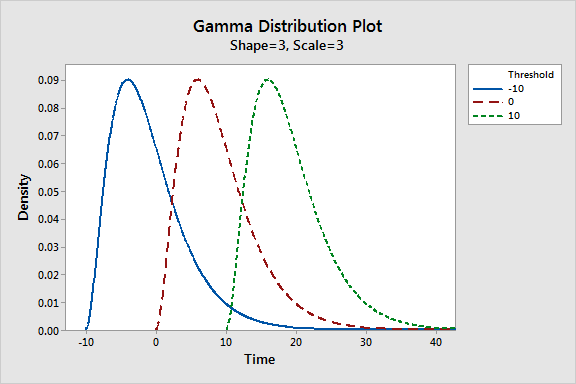
The threshold defines the smallest value in a gamma distribution. Some analysts refer to this parameter as the location. All values must be greater than the threshold. Negative threshold values allow the distribution to handle both negative and positive values. Zero lets it have only positive values. A two-parameter gamma distribution simply has the threshold set to zero.
Holding the shape and scale parameters constant, the threshold shifts the distribution left and right. In the probability distribution plot below, I show the threshold’s effect in action!
Shape Parameter (α)
The shape parameter for the gamma distribution specifies the number of events you are modeling. For example, if you want to evaluate probabilities for the elapsed time of three accidents, the shape parameter equals 3. Shape must be positive, but it does not have to be an integer. Statisticians denote the shape parameter using alpha (α).
The plot below shows how changing the shape parameter affects the distribution while holding the other parameters constant.

Notice how increasing the shape causes the elapsed times to increase. That makes sense because, keeping everything else constant, you’d expect the length of time to grow when you increase the number of events. For example, three accidents (α = 3) will take longer to occur than one (α = 1), and five (α = 5) takes longer than 3.
For very high shape values, the gamma distribution approximates the normal distribution, as shown below.

When the shape of a gamma distribution is an integer, it is known as an Erlang distribution. Analysts frequently use the Erlang distribution in queuing theory.
Scale Parameter (β)
The scale parameter for the gamma distribution represents the mean time between events. Statisticians denote this parameter using beta (β).
For example, if you measure the time between accidents in days and the scale parameter equals 4, there are four days between accidents on average.
Rate Parameter (λ)
Alternatively, analysts can use the rate form of the scale parameter, lambda (λ), for the gamma distribution. Lambda is also the mean rate of occurrence during one unit of time in the Poisson distribution. Use the following equations to convert between the scale (β) and rate (λ) forms:
- β = 1 / λ
- λ = 1 / β
They are reciprocals. To understand why let’s return to our example of one accident occurring every four days on average (β = 4). An equivalent way to state it is that an average of one-quarter accident occurs during one day (λ = 1 / 4 = 0.25).
Effect of Changing the Scale on the Gamma Distribution
The scale parameter represents the variability present in the gamma distribution. Higher values cause the distribution to expand further right and decrease the height. Conversely, lower values contract the distribution to the left and increase its peak.
Alternatively, if you use the rate form of the parameter, higher rates shrink the distribution while lower rates spread it out.
The relationship between the scale parameter and the spread of the gamma distribution makes sense when you understand that the scale represents the mean time between events. When the time between events is longer, the probabilities for prolonged times logically increases. In the graph below, I illustrate this by modeling probabilities for the 4th event (shape = 4) and varying the average times between events.

This graph looks similar to the chart comparing shape parameters. While increasing the shape and scale parameters will both extend the elapsed times, the shape parameter can genuinely change the shape in ways that the scale cannot. For instance, the shape parameter can change the distribution so it looks like the exponential and normal distributions. The scale parameter can only stretch out the distribution that the shape defines.
Related post: Measures of Variability
Comparing the Gamma Distribution to Other Distributions
The gamma, exponential, and Poisson distributions all model different characteristics of a Poisson process. A Poisson process has independent events occurring at a constant mean rate. All these distributions can use lambda as a parameter, which represents that average rate of occurrence. Here’s how these three distributions compare.
The gamma distribution models the time between events. Time is a continuous variable, and the gamma distribution is, likewise, a continuous probability distribution. Conversely, the Poisson distribution models the count of events within a set amount of time. A count is a discrete variable and the Poisson distribution is a discrete probability distribution.
The gamma and exponential distributions are equivalent when the gamma distribution has a shape value of 1. Remember that the shape value equals the number of events and the exponential distribution models times for one event. Therefore, a gamma distribution with a shape = 1 is the same as an exponential distribution.
For example, a gamma distribution with a shape = 1 and scale = 3 is equivalent to an exponential distribution with a scale = 3.

Related posts: Poisson Distribution and Exponential Distribution

Thanks for the quick reply. I have the recently released second edition “SMRD2”. It is excellent, like all of Meeker’s work. It minimally covers goodness of fit tests (4 pages). JT
Hello Jim. Excellent post. I am teaching undergrad/grad students Statistical Methods I. I have been asked by grad students to help them with reliability analysis on several occasions. University students and faculty have access to JMP Pro software at a very nominal cost. I use the JMP help for reliability and web searches to work on these types of problems. Can you recommend reference texts that cover Log Normal, Weibull, Gamma, and Beta distributions at a Masters level? Also, any good reference texts on performing Goodness-Of-Fit tests for the Weibull and Gamma distribution. John Twist, WVU, Morgantown, WV.
Hi John,
Unfortunately, I don’t have a specific reference that I know for sure will cover all those topics. You might look at the following book to see if it’s suitable.
W.Q. Meeker and L.A. Escobar (1998). Statistical Methods for Reliability Data. John Wiley & Sons, Inc.
Dear sir, Thank you very much. You have done great favour by explaining everything easily. Could you give me the list of book you have in market?
Hi,
I have published the following three books:
You can buy them from Amazon and other online retailers. For more information about them and Amazon links for various countries, go to my web store. You can also get free samples at the link below so you can try before you buy!
My Store – Statistics by Jim
Thanks for asking and I hope provides the information you need!
Jim
Hi, suppose I have a distribution of rainfalls in a particular area. I know the maximum probability density is 0.258675 at a rainfall of 572.929 mm per year.
How do I calculate alpha and beta (and from that the mean rainfall)?
Thanks.
Hi, you’re going to need more data than that. Even if you can assume from subject area knowledge that the rainfall follows a gamma distribution, you still don’t have enough information to estimate the distribution from the mean alone.
I really appreciate someone who tries to explain something in a simple way, like what I saw on this page.
Unless the majority of statistical writers hide important information by using standard definitions, that is.
In general, gamma distribution is explained in a way that is very, very predominant. I think you did a good job of explaining why we should use these parameters in a way that was easy to understand.
In one case. “shape parameter” helps me see “what shapes do” rather than “physical body” of the distribution.
Just discovered this great site. Will tune in. Starting to understand Gamma function better
How are you? hope u’r doing well
actually i have few question on gamma distribution.
Now currently i’am working with high -frequency of finance data (tick-by-tick stock market data) and i have problem with the missing value in data, which is there ‘zero’ at the time with no transaction . Then i tried to manipulate the data by applying gamma distribution in r, then my question is how to define the value for parameter ? shape and scale for gamma
I had been struggling to understand the gamma distribution until I discover you, sir. You have a gift for explaining complex ideas well. I am grateful to have discovered your site, which I will be using. I am going to buy your books. Thank you!
Hi Miles,
Thanks so much. I really appreciate your kind words. Enjoy the books! 🙂
First of all, you need to consider what the count variable is in physical or biological terms and whether taking an inverse has a meaning. The truncated Gamma distribution (which would be formed by inverting Likert scale counts) has parameters which relate directly to the heat equation and so your rate variable (inverse count variable) should explain the physics of the system being considered (e.g. covid rates (time since onset to end) are related to seasonal local temperature fluctuations (around 20 degrees)). A proportional hazards model with Gamma hazard rate sholud be fitted with appropriate environmental covariates.
I use software provided by the Environmental Protection Agency (EPA) to calculate upper confidence limits of the mean (among other things) for data sets consisting of contaminant concentrations in samples of waste or environmental media. They offer a choice of distribution assumption – normal, gamma, and lognormal, with an option for nonparametric if none of the distributions fit adequately. Sometimes we also need to calculate a lower confidence limit, which the software doesn’t provide, although they provide a hand-calculation method for normal and lognormal distributions (but not for the gamma distribution). I’ve searched the internet for a method to estimate the LCL of the mean of a gamma distribution to no avail. Can you shed some light?
Dear Jim,
again many thanks for this blog post. One question, and I would like to hear your opinion about this. For one study, we had several dependent variables, some were conditionally normally distributed, some were Poisson or negative binomial distributions, since they were count data. But one was a mean score from likert items, which resulted in a likert scale. For the sake of simplicity I assumed it to be continous therefore. But this variable was highly left-skewed. I did not find any useful distribution and I really do not like transforming the data, I just wanted to stay in the realm of GLMs. Therefore, I inverted the scale, so it became right-skewed and analyzed it with a Gamma distribution. The DHARMa package in R (I do not know if you are familiar with it, but it samples/simulates residuals from an ideal model according to your parameters and compares it with your sample residuals), which indicated a good fit. Do you think, this scale inversion is appropriate or do you have any suggestions for a different approach to handle left-skewed, continous, bounded data? Especially in the GLM or even Bayesian realm (I use brms in R)? Thanks for any suggestions.
Best,
Rainer
Hi Rainer,
Offhand, I don’t see anything wrong with your approach. And, I agree, I don’t like transforming variables either, so using the native distribution seems like a plus to me!
Also, remember that for least squares regression, the normality assumption applies to the residuals and not the distribution of the independent variables. I’ve had models with skewed DVs but was able to obtain normal residuals by specifying the correct model (and not transforming the data).
But, if you got good results with your approach, that sounds reasonable to me! The distribution will extend passed the bounds in your data, that can be ok if you get an otherwise good fit and understand that while interpreting results.
I have not done a similar type of analysis, so I don’t have any personal insights. If you analyze individual Likert items instead of an average, you use ordinal logistic regression.
An excellent post, Jim. I occasionally have to deal with modeling counts of events, or time to events, and I’ve never encountered these distributions in my training. A practical example or two (or three) would be helpful, to show how these distributions are utilized in statistical situations. I use SPSS statistical software which might not be the best one to use when dealing with these. Can problems using these distributions be addressed in Excel?
Hi Jerry,
I don’t believe that you can use Excel for these distributions, but I’m not 100% sure because I haven’t looked for that capability specifically.
I like your idea of including examples. I show the examples for several probability distributions in my post Understanding Probability Distributions. The same type of uses would apply to the Gamma distribution. However, over time, I may add examples to this post and the other distributions!
Please Send the link to buy from India
Hello, thanks for writing!
You can buy the ebooks from India in My Webstore
If you want them in print, you can get them from Amazon India. Here is the link for my Introduction to Statistics book on Amazon India. Scroll down to the Frequently bought together section to see my other books.
Thanks and happy reading!