An ordinary least squares regression line represents the relationship between variables in a scatterplot. The procedure fits the line to the data points in a way that minimizes the sum of the squared vertical distances between the line and the points. It is also known as a line of best fit or a trend line.
In the example below, we could look at the data points and attempt to draw a line by hand that minimizes the overall distance between the line and points while ensuring about the same number of points are above and below the line.

That’s a tall order, particularly with larger datasets! And subjectivity creeps in.
Instead, we can use ordinary least squares regression to mathematically find the best possible line and its equation. I’ll show you those later in this post.
In this post, I’ll define a least squares regression line, explain how they work, and work through an example of finding that line by using the least squares formula.
What is an Ordinary Least Squares Regression Line?
Ordinary least squares regression lines are a specific type of model that analysts frequently use to display relationships in their data. Statisticians call it “least squares” because it minimizes the residual sum of squares. Let’s unpack what that means!
The Importance of Residuals
Residuals are the differences between the observed data values and the least squares regression line. The line represents the model’s predictions. Hence, a residual is the difference between the observed value and the model’s predicted value. There is one residual per data point, and they collectively indicate the degree to which the model is wrong.
To calculate the residual mathematically, it’s simple subtraction.
Residual = Observed value – Model value.
Or, equivalently:
y – ŷ
Where ŷ is the regression model’s predicted value of y.
Graphically, residuals are the vertical distances between the observed values and the line, as shown in the image below. The lines that connect the data points to the regression line represent the residuals. These distances represent the values of the residuals. Data points above the line have positive residuals, while those below are negative.
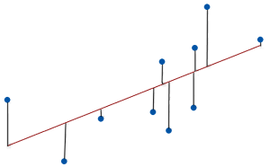
The best ordinary least squares models have data points close to the line, producing small absolute residuals.
Minimizing the Squared Error
Residuals represent the error in a least squares model. You want to minimize the total error because it means that the data points are collectively as close to the model’s values as possible.
Before minimizing error, you first need to quantify it.
Unfortunately, you can’t just sum the residuals to represent the total error because the positive and negative values will cancel each other out even when they tend to be relatively large.
Instead, ordinary least squares regression takes those residuals and squares them, so they’re always positive. In this manner, the process can add them up without canceling each other. Statisticians refer to squared residuals as squared errors and their total as the sum of squared errors (SSE), shown below mathematically.
SSE = Σ(y – ŷ)²
Σ represents a sum. In this case, it’s the sum of all residuals squared. You’ll see a lot of sums in the least squares line formula section!
For a given dataset, the least squares regression line produces the smallest SSE compared to all other possible lines—hence, “least squares”!
Ordinary Least Squares Regression Line Example
Imagine we have a list of people’s study hours and test scores. In the scatterplot, we can see a positive relationship exists between study time and test scores. Statistical software can display the least squares regression line and its equation.

From the discussion above, we know that this line minimizes the squared distance between the line and the data points. It’s impossible to draw a different line that fits these data better! Great!
But how does the ordinary least squares regression procedure find the line’s equation? We’ll do that in the next section using these example data!
How to Find an Ordinary Least Squares Regression Line
The regression output produces an equation for the best fitting-line. So, how do you find an ordinary least squares regression line?
First, I’ll cover the formulas and then use them to work through our example dataset.
Ordinary Least Squares Regression Line Formulas
For starters, the following equation represents the best fitting regression line:
y = b + mx
Where:
- y is the dependent variable.
- x is the independent variable.
- b is the y-intercept.
- m is the slope of the line.
The slope represents the mean change in the dependent variable for a one-unit change in the independent variable.
You might recognize this equation as the slope-intercept form of a linear equation from algebra. For a refresher, read my post: Slope-Intercept Form: A Guide.
We need to calculate the values of m and b to find the equation for the best-fitting line.
Here are the ordinary least squares regression line formulas for the slope (m) and intercept (b):

Where:
- Σ represents a sum.
- N is the number of observations.
You must find the slope first because you need to enter that value into the formula for calculating the intercept.
To find the correct solution, you must use the correct order of operations in the formula. If you need a refresher on that, read my post PEMDAS Explained: Order of Operations in Math.
Worked Example
Let’s take the data from the hours of studying example. We’ll use the ordinary least squares regression line formulas to find the slope and constant for our model.
To start, we need to calculate the following sums: Σx, Σy, Σx2, and the Σxy. We need these sums for the formulas. I’ve calculated the sums, as shown below. Download the Excel file that contains the dataset and calculations: Least Squares Regression Line example.

Next, we’ll plug those sums into the slope formula.

Now that we have the slope (m), we can find the y-intercept (b) for the line.

Let’s plug the slope and intercept values in the ordinary least squares regression line equation:
y = 11.329 + 1.0616x
This linear equation matches the one that the software displays on the graph. We can use this equation to make predictions. For example, if we want to predict the score for studying 5 hours, we simply plug x = 5 into the equation:
y = 11.329 + 1.0616 * 5 = 16.637
Therefore, the model predicts that people studying for 5 hours will have an average test score of 16.637.
Learn how to assess the following ordinary least squares regression line output:
- Linear Regression Equation Explained
- Regression Coefficients and their P-values
- Assessing R-squared for Goodness-of-Fit
For accurate results, the least squares regression line must satisfy various assumptions. Read the following posts to learn how to assess these assumptions:

The issue is not which methodology would fit “better”, but which methodology is more sound from a scientific perspective. Statistical niceties are not relevant for doing science.
That is incorrect. If you’re using data to draw conclusion about reality, you need a good model. It’s not a “nicety”, it’s a requirement. You also need to understand the model that works best given the nature of your data. Case closed.
In my opinion, instead of using minimizing the sum of the least squares, everyone should use the minimum least absolute differences, because the least squares approach each data point differently in the minimization process for no scientifically valid reason. Why minimizes squares of differences, why not raise the difference to the third or fourth power. None of these is justified because they weight different data points differently. It was only a more convenient mathematical technique to solve the least squares approach which led to it dominance, but that is not a valid reason to use it when doing science.
Hi Richard,
Don’t think of it as treating data differently. Instead, it’s choosing the model that best fits your data by understanding the properties of your data.
If the errors in your model are symmetrical (equally likely to be negative and positive) and small errors are much more probable than large errors (in nonlinear decreasing manner), then OLS provides the best fitting model (most precise estimates with no bias). You need to assess your residuals to see if the follow a normal distribution.
The reason OLS is widely used is not just historical convenience. It is optimal under certain conditions (normally distributed errors, homoscedasticity, and no multicollinearity), giving the best linear unbiased estimates (BLUE). If the errors are normally distributed, minimizing squared errors aligns with maximizing the likelihood under a normal error distribution. See my post about the Gauss-Markov theorem.
However, if your errors are symmetrical but larger errors are linearly less likely to occur than smaller errors, then least absolute difference (LAD) might fit better. More specifically, LAD is more appropriate when errors follow a Laplace (double exponential) distribution rather than a normal distribution.
Additionally, if you have outliers that you cannot remove, this approach can be more robust to outliers because it does not excessively penalize large deviations. However, note the tradeoff. LAD estimates have higher variance compared to OLS when the normality assumption holds (i.e., less precise estimates).
It comes down to understanding your data and the model that best fits them. Consider using LAD when you have heavy-tailed distributions and heteroscedastic data. Checking your residuals can help you make that decision.
I’m aware of your particular circumstances, so I’ll just note that this approach is the best general approach. I don’t know the answer for your particular case.
Best wishes,
Jim
Jim,
Thank you for the response.
The one thing I forgot to say in my initial question(s) was that when completing a market condition/time adjustment for appraisals I am not utilizing inferential statistics as I am not choosing a sample to project to a greater population.
The key is to truly search for properties that compete/are comparable to my subject. Once I have that data set that is my market segment.
Having controlled the data by minimizing the property size, acreage, etc.. of the search parameters, I have minimized the noise in the data and from there only utilizing descriptive statistics as I am only looking to derive the trend for my competing market segment.
Jim,
I have read two of your books – Regression Analysis and Thinking Analytically, and I find myself referencing the Regression Analysis book on a regular basis.
I have corresponded with you in the past, but it has been some time. I am a real estate appraiser and primarily utilize linear regression in deriving market condition time adjustments.
I control my data by narrowing my property searching parameters to minimize the noise in the data. If my property is 2,000 square feet, and on a quarter acre, I might narrow my search to properties that sold within the past year between 1,800 and 2,300 square feet, with a lot size up to an acre.
I typically utilize a linear trend line, and then, depending on where/how the data points fall in relation to the linear line on the scatter plot, will put on a quadratic or cubic trend line.
My question to you is, in practical terms, is there any time where a 4th, 5th, or higher polynomial trend line would be relevant? I see people putting high level trend lines on plots all the time, but to me they are not really reflecting the data; rather they are reflecting the “noise” that remains in between the data.
When I see a change in trends I typically move to create two separate scatter plots – a spline linear – so I can model the straight line changes at each point in time. In your opinion, would that be an accurate way of modeling a sale price trend?
Lastly, I tend to shy away from utilizing/modeling median sale prices when I have all of the sales. Utilizing the median one looses the individual sales prices and sales dates (data points) and I have found that the median can actually reflect the trend in the opposite direction.
Sorry for the long message. Any insight you can provide or comment on would be greatly appreciated.
Thank you,
Ed Bedinotti
Hi Ed,
I’m so glad to hear that you’ve found my books to be helpful!
First, about higher-order polynomials. I share your concerns about them! In practice, I’ve only found squared terms to be realistic. Occasionally, I’ve seen cases where a cubic term sort of works but the curve actually requires a truly nonlinear model (polynomials work within linear models even though they fit curvature, which you know having read my book!). I would suspect that you’re correct that using even higher order terms is simply modeling the error (aka overfitting the model). You’d have to have a strong theoretical reason for fitting those terms.
I guess my primary concern about narrowing property parameters that would would be reducing the sample size and allowing chance fluctuations to play a larger role. You might also accidentally exclude large trends that happen not exist in your specific sample. Also, just be aware that when you have a correlation between say property size and price, if you restrict the range of values on one side of the correlation (i.e., property size), you will weaken or eliminate the strength of the correlation. While you are focused on property values, just be aware that any correlations you’re looking at in such highly filtered data might be weakened.
I think your spline approach is probably ok. And I only say “probably” because I’m not an expert in real estate and don’t know the ins and outs of analyzing that data. Splines are a good way to avoid using higher-order polynomials, particularly when the data show different trends over periods. Splines are particularly good when there are abrupt changes in the trends. If that sounds like your data, then it’s probably a good choice. If the trends change smoothly and continuously, you might want to instead model with a potentially nonlinear model. But if you really need the model to fit specific section of the data well, splines are probably what you should use. If you need an excellent overall equation for all the data, I’d try fit a single (potentially nonlinear) model.
I hope that answers your questions! Thanks for writing!
Jim
Hi Jim,
Happy new year!
In your book you describe centering the data to achieve a more reliable constant in OLS regression. Why does centering produce a more reliable constant? I do it all the time now. It does not seem to make sense, Why should regressing the y-variable corrected for the Y-average produce a more meaningful constant?
Hi Stan,
Happy new year to you as well!
Centering all the continuous variables in a linear regression model is beneficial for several reasons, some of which relate to the constant. It also helps reduce structural multicollinearity when you include polynomial and interaction terms. But I’ll focus on the constant here and two main reasons. Prepare for a long reply!
First, by centering the continuous variables, the constant represents the mean response when all the continuous variables are at their mean values (and any categorical variables are at their baseline value). That’s a benefit because it guarantees that your model estimates the constant using actual data values that are in range of what’s being estimated. In other words, you’ll undoubtedly have actual observations occurring with the variables near their mean values. Your estimate for the constant is based on data values that actually exist in your dataset.
Now, compare that to uncentered data where the constant represents all the continuous variables at their zero values simultaneously. Depending on your subject matter, it might be unrealistic to have all your predictors at zero simultaneously. Or, it might realistic for some but not all. It some cases, zero values can be impossible depending on what you’re measuring. The end result for any of these cases is that you’re estimating a constant for either an impossible condition or one that didn’t occur in your dataset. You’re estimating something that is outside the range of your data, which is always risky. Conversely, when you center the data, you’re guaranteeing that your estimating within the range of your data.
The second point builds on the first. When you estimate outside the range of the data, your estimate is less reliable. The relationship between the variables can change across different ranges of values. Your model only estimates the relationships between variables for the range of data values in your dataset. If the relationship changes outside your observed data range, extrapolating outside that range will produce inaccurate results. Your relationships can be locally linear, but nonlinear over larger ranges. In the context we’re talking about, it means your constant is unreliable because the data for that point don’t exist in your dataset.
I show an example of that using body weights in the book using simple regression. The relationship between height and weight is linear in the data range I use for the model starting on page 68 but the value for zero height is outside the data range. The relationship for the range I have is locally linear. However, we can deduce that is nonlinear when you expand the age range, particularly looking at birth weights. That’s why the model I use gives a negative value for the constant. A negative weight is clearly impossible. It was calculated using values outside the actual data range because there was no height value of zero in the dataset. Indeed, a height of zero is impossible in this case!
In short, the constant represents a negative weight for a height of zero, which makes no sense for either variable in this context. Nor do we even have height data near zero, so the model is estimating the constant outside the range of the data. In other models, perhaps the zero values make sense but don’t exist in the dataset. That’s still problematic in terms of interpreting the constant because the conditions the constant represents is outside the range of observed data.
When I refit the model on page 74 by centering heights, we guarantee that zero height values, which now represent the mean height, are in the dataset. That means the new constant is estimated using values within the range of the actual data. We’re not estimating outside the data range.
It’s also more interpretable because now the constant represents the mean weight for the average height in the dataset. That makes much more sense and is based on data that are in the dataset.
There might be some cases where having zero values for all your predictors simultaneously both makes sense and exists in your dataset. In those cases, you might not need to center the data. In practice, I’ve found that has never happened for me. However, in some subject areas, it could be more common. Let your data guide you on that!
I will say that even if you don’t center the data but have a good model that fits the data, you might not be able to interpret the constant but the rest of your model should be good. So, it’s not like uncentered models are bad all around, you just might not be able to interpret the constant.
Jim,
Thank you for the reply. I understand it
Stan Alekman
Hi Jim, thanks a lot for your explanations. In another section you explain the interpretation of coefficients for a linear regression. I am not very clear on the interpretation of coefficients in the case of linear regression with bucketed variables (binning) and target encoding for independent variables. Let’s say I have two variables: country and gender. I group the most similar distinct values in terms of the target variable (historical saving rate of candidates, in my case) into buckets for each of these two variables. These will be the input variables in the regression.
For example, the average saving rate in the US and Canada is 60%. Thus, the dependent variable (y) is the historical saving rate of each individual and the independent variable (x) is the average value of historical saving rate for each separate bucket.
You wrote, “The coefficient value signifies how much the mean of the dependent variable changes given a one-unit shift in the independent variable while holding other variables in the model constant.” For example, does a coefficient of 0.5 indicate that the mean saving rate in these countries will change by 0.5% when the average saving rate changes by 1%? I am not sure if my understanding of this sentence for my regression is meaningful.
Additionally, I am not sure how I should assess the goodness of the regression. Does R-squared make sense for such a type of regression, given that the independent variable is an average value of the dependent variable?
Thanks for your explanation, Jim, but you have ignored my basic point which is in doing science, different data points should not be given different (unknown) weights via the squaring process. To me that takes precedence over any mathematical considerations with respect to normal distributions and what you call biased results. The best results are those that do not given give different data points different weights in the first place.
Hi Richard,
I answered your question. Least squares regression provides the most precise, unbiased estimates for linear regression when you can satisfy all the assumptions. It considers all data points using the same algorithm. Generally, when you’re performing an analysis, you want the best results possible. That’s why you’d use it.
We can take a look at your concerns about “different weights.” First of all, not all regression involves people. Secondly, you seem to prefer LAD regression but that also weights observations differently. Outliers are still counted more than those closer to the mean. It’s a linear vs. nonlinear function but both count more extreme observations more heavily the further out they are. Crucially, both methods use relevant characteristics of the observation towards that end and not some arbitrary criteria. Just be aware that LAD also weights observations differently.
But that’s not a problem. Let’s take a look a the field of medicine. Suppose you have two patients and, based on relevant characteristics of both patients, one has risk factors for a disease while the other does not. For best results, the doctor will treat the patients differently based on relevant criteria. Similarly, least squares and LAD regression take the relevant characteristics and handles them accordingly. Treating everyone the same doesn’t always work best in both medicine and regression. You need to treat them appropriately based on relevant criteria.
That’s what least squares and LAD regression do.
What you should focus on instead is whether least squares or LAD is more appropriate for your data given its characteristics. If your dataset has outliers that you can’t remove, consider LAD amongst other possibilities. If you can satisfy all the assumptions of least squares, use it.
Alternatively, you could perform a special study involving only the outliers. Maybe they’re a separate population requiring a specific study?
Those are more pertinent and productive questions than just criticizing least squares. Least squares is good for some cases while other methods are better for others. You need to make that determination.
First of all most real world data in not normally distributed, and one certainly should not assume that it is for the purpose of doing science, namely trying to find causes and effects. Secondly, therefore, the mathematical properties of least squares methods are not relevant to doing science, which means analyzing the data as it comes. Third, in doing science, as far as I can see, there is absolutely no rationale for weighting different data points differently as a function of how far they end up lying from the regression line. Can you give me a rationale? For example, when doing regression analysis for epidemiology, each data point is a person, and all people’s data should be considered equally!!!
Hi Richard,
You seem a little bent out of shape over the normal distribution! So, my first suggestion is to calm down.
I explained the rationale for using squared differences in least squares in my previous reply. Go back and reread that.
From a mathematical standpoint, using the least squares method provides the best coefficient estimates (unbiased, lowest variance) for linear models when the error term is normally distributed. That’s a factual statement from a mathematical perspective. The mathematical properties ARE relevant when you’re using regression to analyze your data assuming you want to obtain trustworthy results.
Your point about the prevalence of the normal distribution is a separate issue. Regardless of the normal distribution’s prevalence, it doesn’t change the mathematical truth behind the least squares method, it just affects how often you can apply it.
I’m not going to debate you on that but I’ll provide my perspective. For starters, the normality assumption for least squares regression applies to the residuals, not the distribution of the variables. You can have nonnormal variables but still produce normally distributed residuals.
As for the variables, or the phenomena themselves, in my extensive experience in the field, I’m surprised at how often data fit the normal distribution. And, in regression, you frequently can obtain normally distributed residuals. However, that’s not always true. For instance, while human heights are normally distributed, weights are not. I suspect that some fields deal with nonnormal data more than others.
But this property is something you can check. I’m not sure where you got the idea that you just assume data or residuals follow a normal distribution. You can check it using distribution tests (e.g., normality tests). And I always point out the importance of checking residual plots after performing regression analysis. One of the reasons to see whether they are normally distributed!
So, it’s not guaranteed whether your variables or residuals follow the normal distribution. You need to check that out. But, if you can obtain normally distributed residuals and satisfy the other least squares assumptions, then from a mathematical standpoint you will get the best results using the least squares method. Period.
If you have significant outliers in your data that you can’t remove, then consider LAD regression as one of the possible remedies. But it’s a specialized method that is only good for certain cases.
Yes, your data comes in however it is. But you must choose the correct statistical methods based on your data’s properties. Failure to do that can distort your results.
Why don’t you favor least absolute differences for regression analysis instead of least squares? Why should points farther from the regression line have much greater impact on where the line is located?
Hi Richard,
That’s a great question!
The least squares differences approach better aligns with the normal distribution. Consider that in the bell-shaped curve, two-thirds of the observations fall within +/- 1 standard deviation from the mean. So a 2 SD range contains about 2/3 of the values. Now take the range of -1 SD to infinity plus the range of + 1 SD to infinity, which I show in the image below for clarity. That massive range contains only 31.74% of the observations. Only only 4.55% of values are more extreme that +/- 2 SD.

This non-linear drop-off means that extreme values (outliers) are much, much rarer than values close to the mean. Least squares regression leverages this property by squaring the residuals, which penalizes larger deviations more severely. This results in a regression line that is heavily influenced by outliers, aligning well with the assumption of normally distributed errors.
In contrast, least absolute differences (LAD) regression minimizes the sum of the absolute values of the residuals. This method treats all deviations equally, regardless of their magnitude. While LAD is less sensitive to outliers, making it useful in cases with significant outliers, it does not align as closely with the characteristics of the normal distribution.
Least squares regression is preferred in many cases due to its mathematical properties, such as producing the best linear unbiased estimators (BLUE) under normally distributed errors. However, for data with many outliers LAD regression or other robust methods may be more suitable.
I hope that helps!
its wonderful. Very well explained..
Amazing sir , no words for the explanation.