What is the Law of Large Numbers in Statistics?
The Law of Large Numbers is a cornerstone concept in statistics and probability theory. This law asserts that as the number of trials or samples increases, the observed outcomes tend to converge closer to the expected value.
Whether you’re a student, a professional statistician, or just someone fascinated by the intricacies of probability, understanding the Law of Large Numbers is crucial. In this comprehensive post, we’ll explore both the weak and strong forms of this law, simulate real-world examples, and uncover why these principles are indispensable in statistics and probability.
By the end of this article, you’ll have a clearer understanding of how the Law of Large Numbers operates in various scenarios and why it’s a key player in predicting and understanding random events.
Exploring the Two Forms of the Law of Large Numbers
There are two forms of the law of large numbers, but the differences are primarily theoretical. The weak and strong laws of large numbers both apply to a sequence of values for independent and identically distributed (i.i.d.) random variables: X1, X2, …, Xn.
Weak Law
The weak law of large numbers states that as n increases, the sample statistic of the sequence converges in probability to the population value. Statisticians also refer to this form of the law as Khinchin’s law.
Here’s what that means. Suppose you specify a nonzero difference between the theoretical value and the sample value. For example, you might define a difference between the theoretical probability for coin toss results (0.50) and the actual proportion you obtain over multiple trials. As the number of trials increases, the probability that the actual difference will be smaller than this predefined difference also increases. This probability converges on 1 as the sample size approaches infinity.
This idea applies even when you define tiny differences between the actual and expected values. You just need a larger sample!
Strong Law
The strong law of large numbers describes how a sample statistic converges on the population value as the sample size or the number of trials increases. For example, the sample mean will converge on the population mean as the sample size increases. The strong law of large numbers is also known as Kolmogorov’s strong law.
Both laws apply to various characteristics, ranging from the means for continuous variables to the proportions for Bernoulli trials. I’ll simulate both of these scenarios next!
Practical Simulations for Demonstrating the Law of Large Numbers
While there are mathematical proofs for both laws of large numbers, I will simulate them using my favorite random sampling program, Statistics101! You can download it for free.
Here are my scripts for the IQ example and the coin toss example. You can perform the simulations yourself and see the results. I include example graphs below that I created using these scripts. I exported the data into Excel for prettier graphs, but Statistics101 produces graphs too. Your simulations won’t match mine, but they should follow the same overall pattern that I discuss.
IQ Example
Imagine that we’re studying IQ scores. We are randomly selecting 100 participants and measuring their IQs. As we gather subjects, we’ll assess their IQ and then recalculate the sample mean with each additional person. This process produces a sequence of sample means as the sample size increases from 1 to 100. If the law of large numbers holds true, we’d expect the sample means to converge on the population mean as the sample size increases. Let’s see!
For this population, I’ll define the population distribution of IQ scores as following a normal distribution with a mean of 100 and a standard deviation of 15.

As you can see, the sample means converge on the population mean IQ value of 100. At the beginning of the sequence, they’re more erratic, but they stabilize and converge on the correct value as the sample size increases.
Coin Flipping Example
Now, let’s look at coin flips. This is a Bernoulli Trial because there are precisely two outcomes, heads or tails. The data are binary and follow the binomial distribution defined by a proportion of events. For this scenario, we’ll define an event as heads in the coin toss. A coin toss is one trial. The law of large numbers predicts that as the number of trials increases, the proportion will converge on the expected value of 0.50.

It works! The sample proportion become more stable and converges on the expected probability value of 0.50 as the sample size increases.
Practical Implications of the Law of Large Numbers
The law of large numbers is essential to both statistics and probability theory.
For statistics, both laws of large numbers indicate that larger samples produce estimates that are consistently closer to the population value. These properties become important in inferential statistics, where you use samples to estimate the properties of populations. That’s why you always hear statisticians saying that large sample sizes are better!
Related post: Inferential versus Descriptive Statistics
In probability theory, as the number of trials increases, the relative frequency of observed events will converge on the expected probability value. If you flip a coin four times, it’s not surprising to get three heads (75%). However, after 100 coin flips, the percentage will be extremely close to 50%. Learn more about Expected Values: Definition, Formula & Finding.
These laws bring a type of order to random events. For example, if you’re talking about flipping coins, rolling dice, or games of chance, you are more likely to observe an unusual sequence of events over the short run. However, as the number of trials grows, the overall outcomes converge on the expected probability.
Consequently, casinos with a large volume of traffic can predict their earnings for games of chance. Their earnings will converge on a predictable percentage over a large number of games. You might beat the house with several lucky hands, but in the long run, the house always wins!
Caution: Inappropriately applying the law of large numbers to the short run can make you a victim of the gambler’s fallacy.
Related post: Fundamentals of Probability
When the Laws of Large Numbers Fail
There are specific situations where the laws of large numbers can fail to converge on the expected value as the sample size or the number of trials increase. When the data follow the Cauchy distribution, the numbers can’t converge on an expected value because the Cauchy distribution does not have an expected value. Similarly, the laws don’t apply to the Pareto distribution because its expected value is infinite.
Significance of the Law of Large Numbers in Probability and Statistics
In summary, the Law of Large Numbers is more than a statistical theory; it’s a fundamental principle that brings order and predictability to the randomness of life’s events. From flipping coins to rolling dice, and from casino games to predicting long-term trends, this law ensures that, over a large number of trials, outcomes will align with theoretical probabilities.
I hope this exploration has deepened your understanding of how large numbers play a pivotal role in bringing certainty to the uncertain world of random events. Keep in mind that larger sample sizes often yield more reliable estimates, echoing the profound implications of this law in statistical practices and everyday decision-making. Stay curious, and continue exploring the fascinating world of statistics and probability!

Hi Jim: Accepting large samples should converge on the population mean or a “best-fit” regression line (my interest is in the latter example), do large numbers also affect the 95% prediction intervals of the regression (not the 95% CI for the regression line, but the 95% prediction intervals for the paired data). Or is the spread (variability) of the data points more relevant to the prediction intervals, regardless of sample size. The question that is debated in our group is that large samples (n>15,000) are all that are needed whereas others point out that while the regression line and its 95% CI are probably close to that of the true population, it is the overall sample variability – not the sample size – that determines the 95% prediction limits for the data (or added data points). Thank you!
Hi,
That’s a great question and an astute one. As you’ve guessed, the role of sample size differs between the confidence interval of the prediction (CI for the mean outcome) versus the Prediction Interval (PI), which predicts the range for a single value. In both cases, it’s a combination of the variability and sample size that affects the widths. However, the role of sample size is less pronounced for PIs. For starters, for any given sample size, the PI will be wider than the corresponding CI of the prediction. Now, let’s look at the roll of sample size conceptually first and then with equations.
As sample size converges on infinity, the widths of CIs converge on zero. That makes sense because if you were to measure an entire population, there’d be zero uncertainty about the population mean (in this case the mean outcome). The mean is based on all the values you’ve already measured and nothing else.
However, if you measured the entire population, you’d still have uncertainty about the next new value added to the population. All the measured variability creates uncertainty around the next new value because you’re predicting something new outside of what you’ve already measured. Consequently, for PIs, as sample size increases, the width narrows more slowly and the minimum width is limited by the variability.
You can see how that works in the two equations.
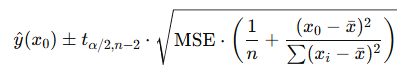
Confidence Interval of the Prediction
Prediction Interval
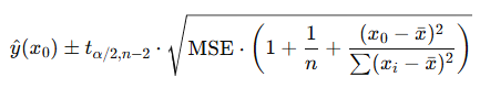
The two equations are nearly identical except for the constant of 1 in the PI formula’s square root. This value represents the irreducible variation in individual values and limits how much the PI can decrease with larger sample sizes.
So, ultimately, yes, variability is the limiting factor for PIs but not for CIs. Consequently, the role of sample size is diminished for PIs. Said another way, if you want a CI of a particular width no matter how narrow, you can just keep increasing sample size until you obtain that width. With PIs, increasing the sample size will help reduce the width but the degree is limited by the variability.
Hello Jim,
Does the Law of Large numbers also applies to dependent events? I’m curious about this because of Markov Chains. Markov Chains uses semi-dependent events or states when calculating the probability of moving from one state to the next state. Another example could be the standards playing cards, like what’s the probability of getting two Aces in a row over a large number of samples. I read somewhere that this law could also apply to dependent events. Is this true? Thank you and have a good day.
Sincerely,
Emikel
Hi Emikel,
I believe it can apply in those cases but you have to be careful in doing so. You need to know exactly what the dependent condition is that affects the next outcome. And then know that the law of large numbers applies to that probability. For example, suppose event B has a 60% chance of occurring if event A occurs, but only a 30% chance if event A does not occur. With a large number of opportunities, you’d expect that the observed frequencies will close in on those theoretical frequencies. But, you’ll need to be careful to know whether A occurs or not and keep track of the results accordingly. Bu, with a large number of outcomes you’d expect the observed frequencies to be close to 60% and 30%, respectively.
I love these topics thanks for sharing!
What are Cauchy distribution and Pareto Distribution ?